v5.1: Three-neutrino fit based on data available in October 2021
Menu
- Summary of data included
- Parameter ranges
- Leptonic mixing matrix
- Two-dimensional allowed regions
- One-dimensional χ2 projections
- CP-violation: Jarlskog invariant
- CP-violation: unitarity triangle
- Tension between Solar and KamLAND data
- Synergies: atmospheric mass-squared splitting
- Synergies: disappearance data and θ23
- Synergies: determination of θ23
- Synergies: determination of δCP
- Synergies: determination of Δm23ℓ
- Correlation between δCP and other parameters
- Available data files
If you are using these results please refer to JHEP 09 (2020) 178 [arXiv:2007.14792] as well as NuFIT 5.1 (2021), www.nu-fit.org.
|
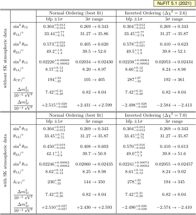
| Three-flavor oscillation parameters from our fit to global data as of October 2021. The results shown in the upper (lower) section are obtained without (with) the inclusion of the tabulated χ2 data on atmospheric neutrinos provided by the Super-Kamiokande collaboration (SK-atm). The numbers in the 1st (2nd) column are obtained assuming NO (IO), i.e., relative to the respective local minimum. Minimization with respect to the ordering provides the same results as Normal Ordering, except for the 3σ range of Δm23ℓ in the analysis without SK-atm. Note that Δm23ℓ = Δm231 > 0 for NO and Δm23ℓ = Δm232 < 0 for IO. |
|
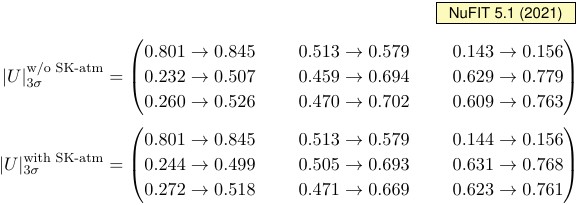
| 3σ CL ranges of the magnitude of the elements of the three-flavor leptonic mixing matrix under the assumption that the matrix U is unitary. The ranges in the different entries of the matrix are correlated due to the fact that, in general, the result of a given experiment restricts a combination of several entries of the matrix, as well as to the constraints imposed by unitarity. As a consequence choosing a specific value for one element further restricts the range of the others. The upper (lower) limits are obtained without (with) the inclusion of the tabulated SK-atm χ2 data. |
Two-dimensional allowed regions
pdf jpg |
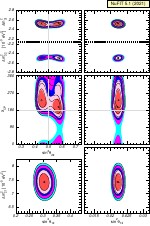
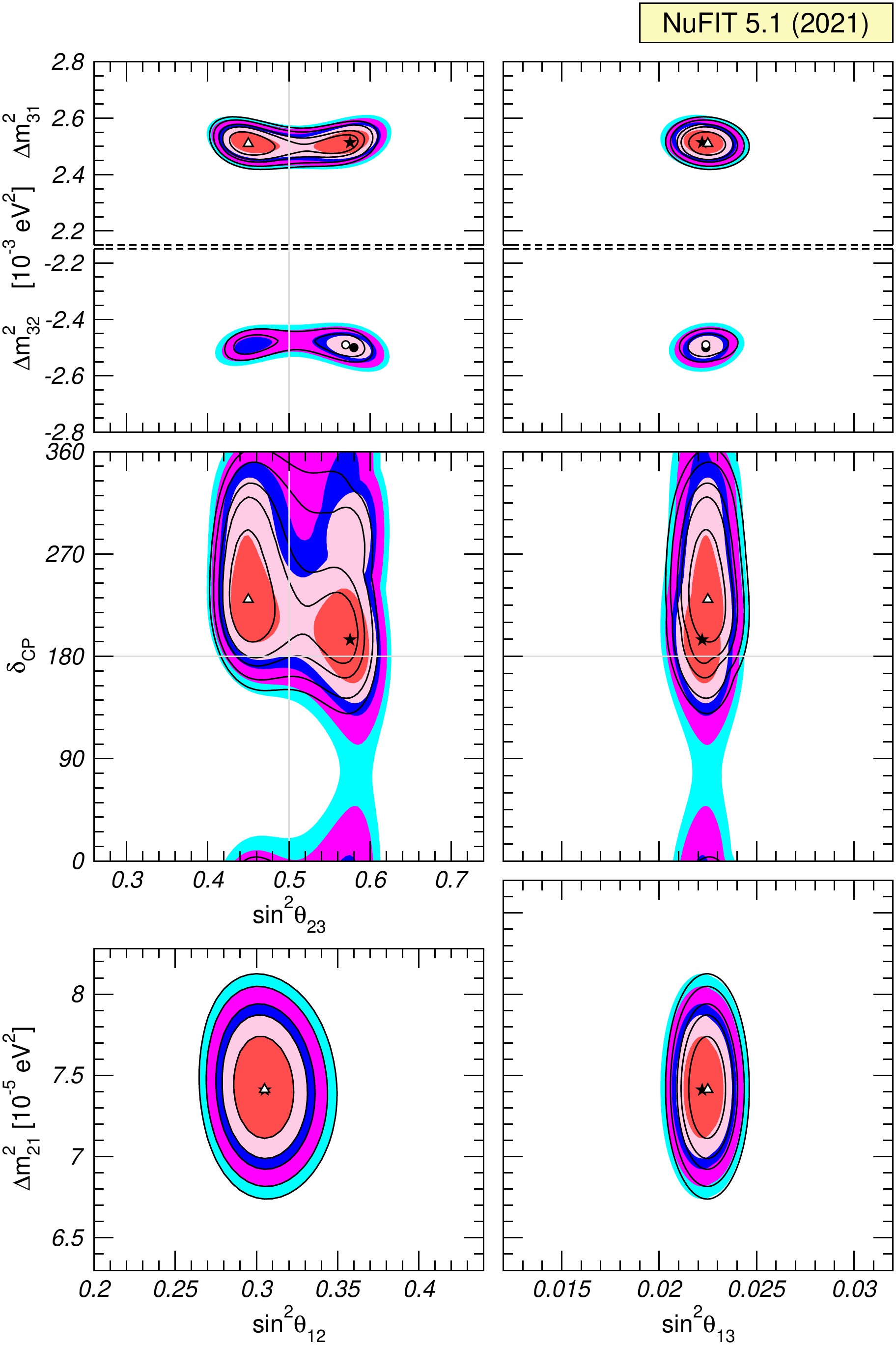
Global 3ν oscillation analysis. Each panel shows the two-dimensional projection of the allowed six-dimensional region after marginalization with respect to the undisplayed parameters. Colored regions (black contour curves) are obtained without (with) the inclusion of the tabulated SK-atm χ2 data. The different contours correspond to the two-dimensional allowed regions at 1σ, 90%, 2σ, 99%, 3σ CL (2 dof). Note that as atmospheric mass-squared splitting we use Δm231 for NO and Δm232 for IO. The regions in the lower 4 panels are based on a Δχ2 minimized with respect to the mass ordering. |
One-dimensional χ2 projections
pdf jpg |
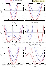
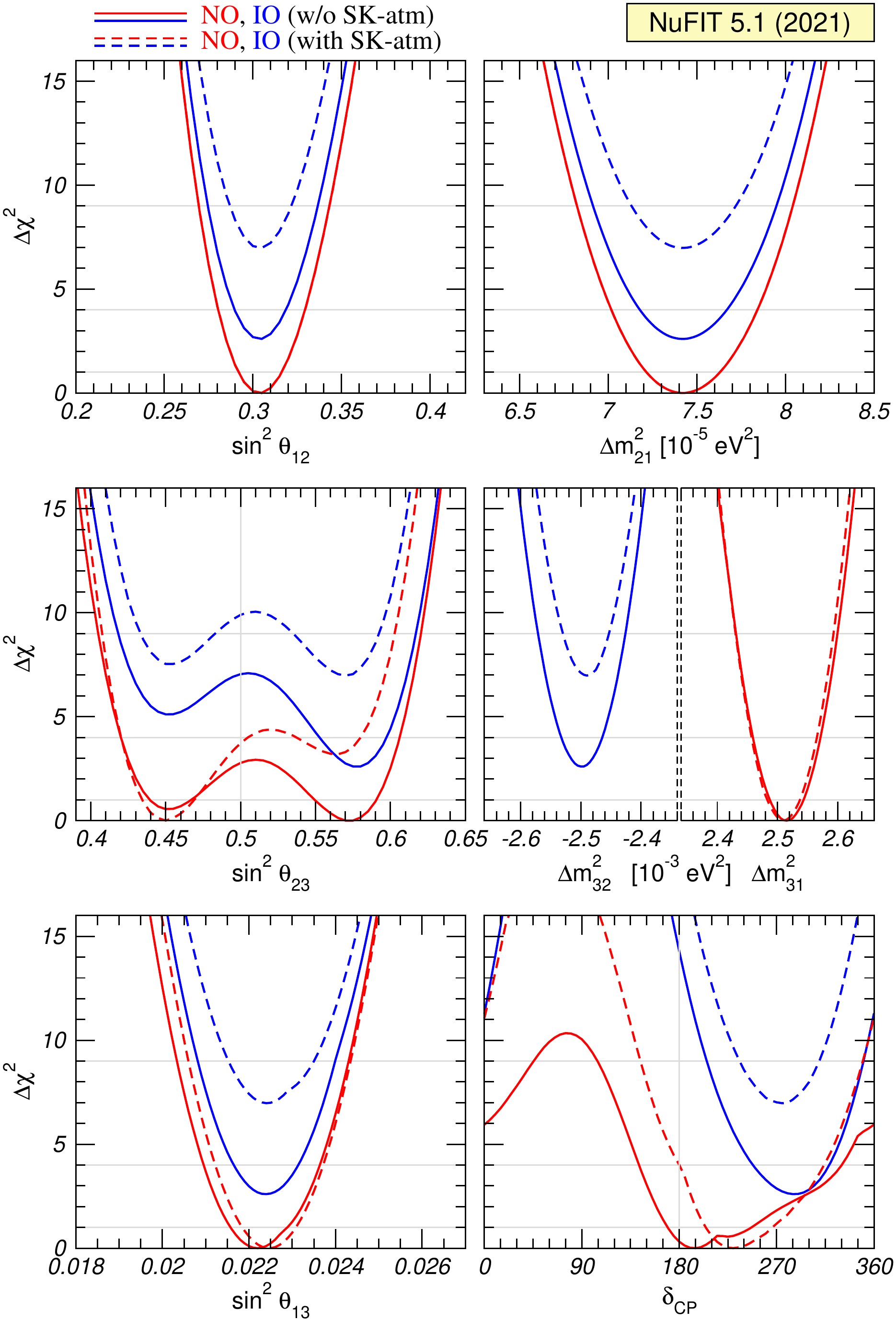
Global 3ν oscillation analysis. The red (blue) curves are for Normal (Inverted) Ordering. The solid (dashed) lines are obtained without (with) the inclusion of SK-atm χ2 data. As atmospheric mass-squared splitting we use Δm231 for NO and Δm232 for IO. |
CP-violation: Jarlskog invariant
pdf jpg |
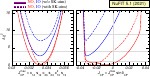
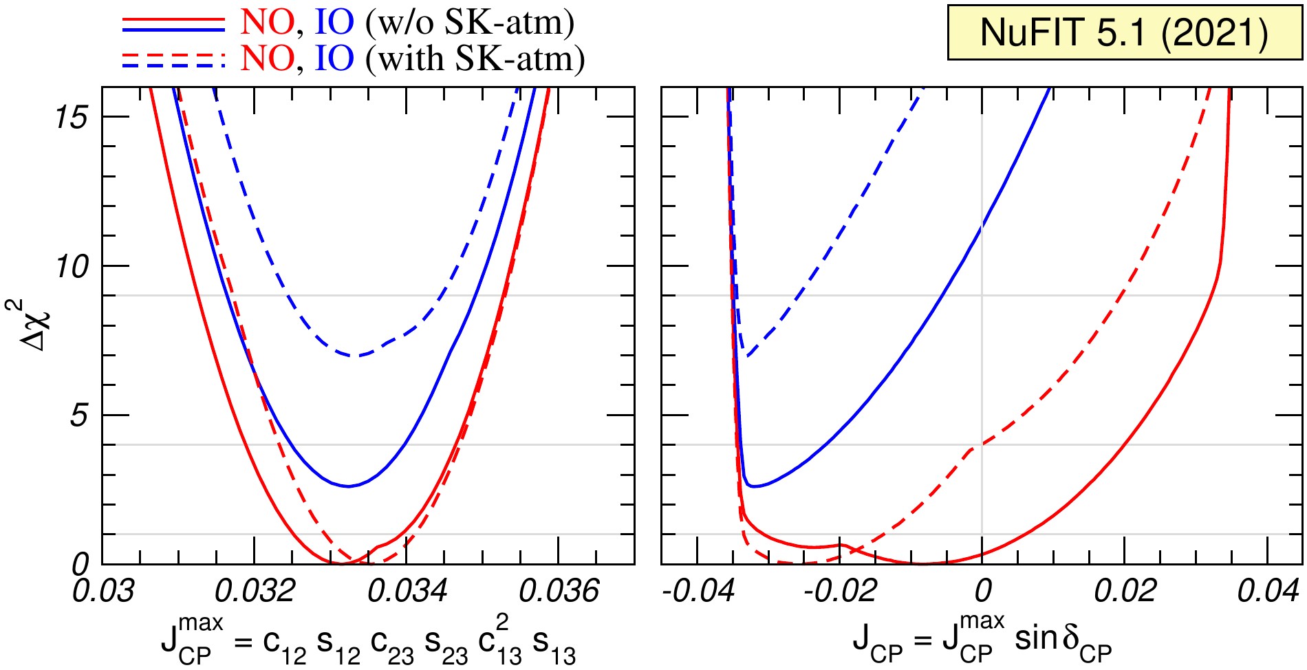
Dependence of Δχ2 on the Jarlskog invariant (right) and its δCP-independent modulus (left). The red (blue) curves are for Normal (Inverted) Ordering. The solid (dashed) lines are obtained without (with) the inclusion of the tabulated SK-atm χ2 data. |
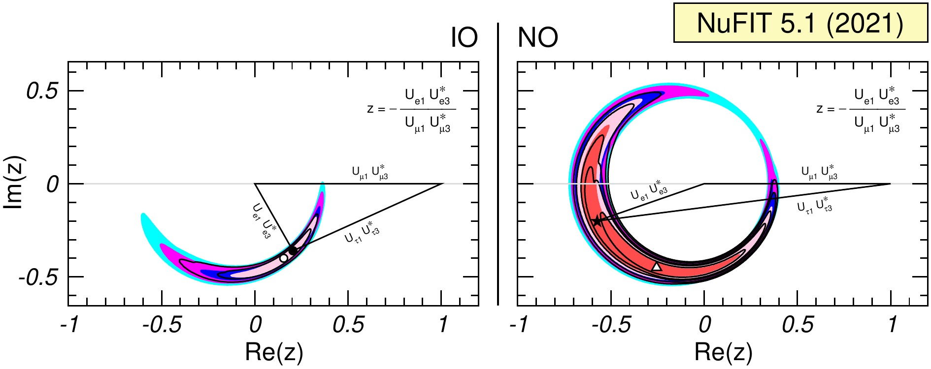
CP-violation: unitarity triangle
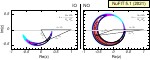
pdf jpg |
Leptonic unitarity triangle for the first and third columns of the mixing matrix. After scaling and rotating each triangle so that two of its vertices always coincide with (0,0) and (1,0), we plot the 1σ, 90%, 2σ, 99%, 3σ CL (2 dof) allowed regions of the third vertex. Colored regions (black contour curves) are obtained without (with) the inclusion of the tabulated SK-atm χ2 data. The contours for Normal (right) and Inverted (left) ordering are defined with respect to the common global minimum. Note that in the construction of the triangles the unitarity of the U matrix is always explicitly imposed. |
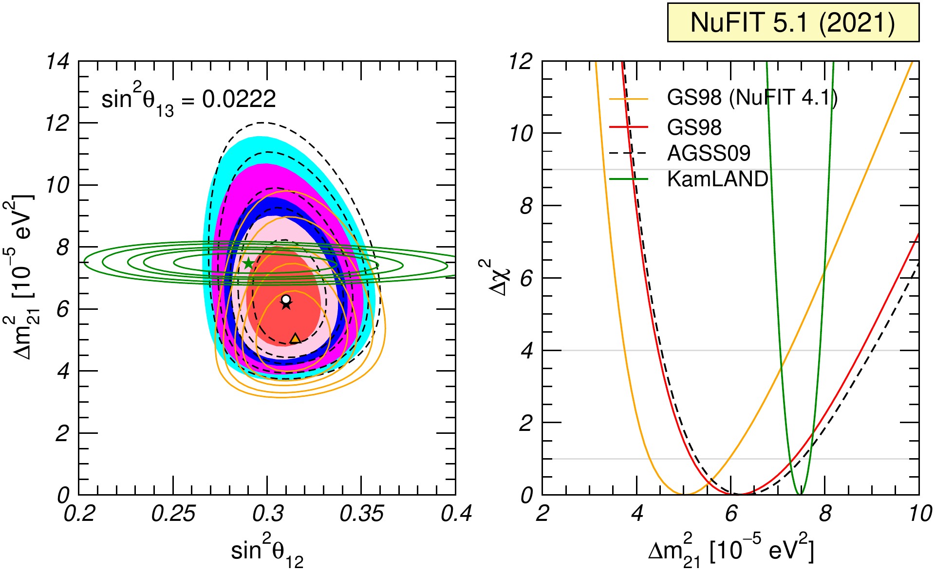
Tension between Solar and KamLAND data
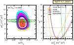
pdf jpg |
Left: Allowed parameter regions (at 1σ, 90%, 2σ, 99%, 3σ CL for 2 dof) for fixed θ13 = 8.6° from the analysis of KamLAND data (solid green contours with best fit marked by a green star) and from the combined analysis of solar data for the GS98 model (full regions with best fit marked by black star) and the AGSS09 model (dashed void contours with best fit marked by a white dot). We also show as orange contours the results of a global analysis for the GS98 model using the previous SK4 neutrino data. Right: Δχ2 dependence on Δm221 for the same four analyses after marginalizing over θ12. |
Synergies: atmospheric mass-squared splitting
pdf jpg |
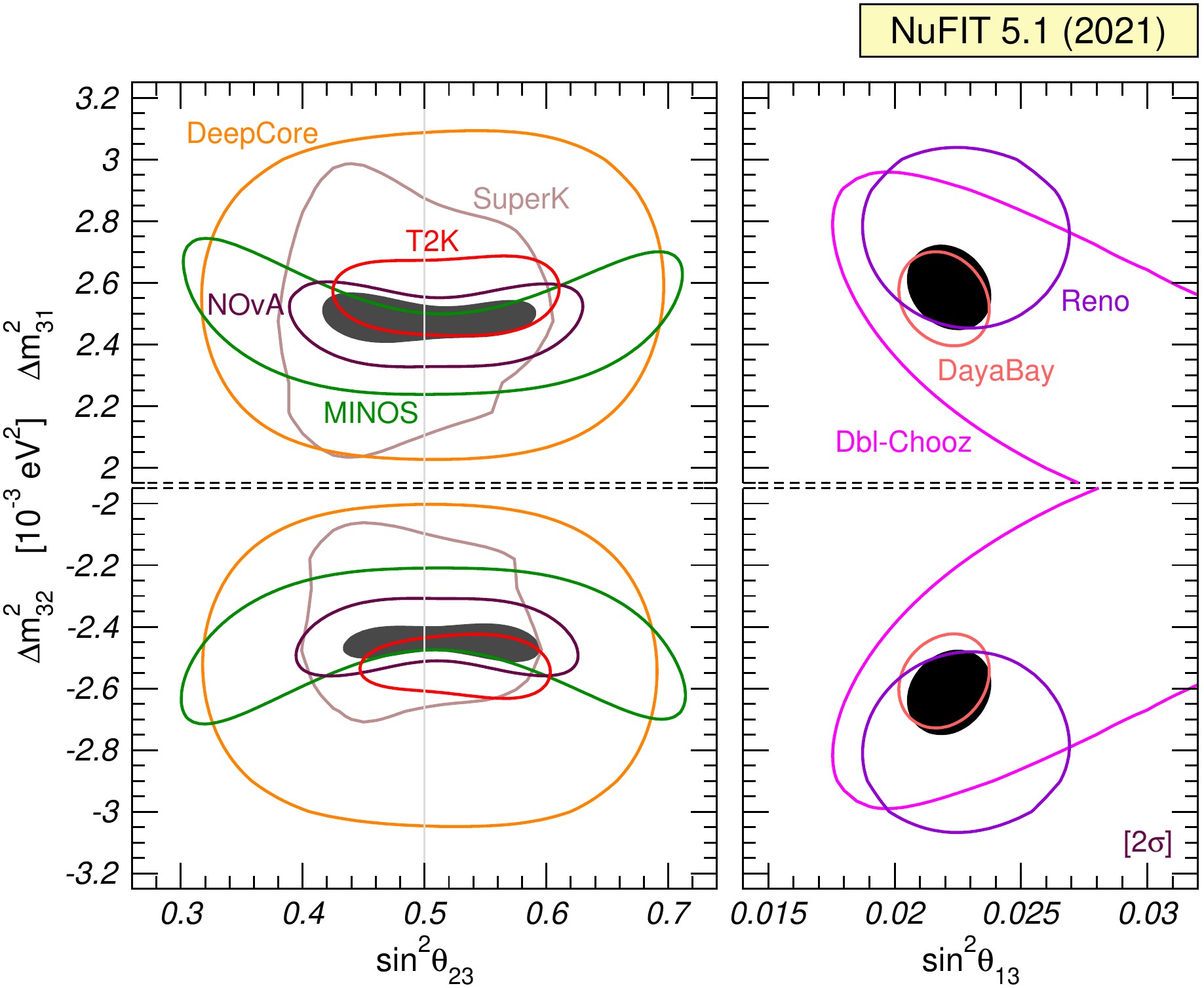
Determination of Δm23ℓ at the 2σ confidence level (2 dof), where ℓ = 1 for NO (upper panels) and ℓ = 2 for IO (lower panels). The left panels show regions in the (sin2θ23, Δm23ℓ) plane using both appearance and disappearance data from MINOS (green), NOνA (dark-redwood) and T2K (red), as well as atmospheric data from DeepCore (orange) and Super-Kamiokande (light-brown), and a combination of all of the above (dark-grey region). Here a prior on θ13 is included to account for reactor bounds. The right panels show regions in the (sin2θ13, Δm23ℓ) plane using data from Daya-Bay (pink), Double-Chooz (magenta), RENO (violet), and their combination (black regions). In all panels solar and KamLAND data are included to constrain Δm221 and θ12. Contours are defined with respect to the global minimum of the two orderings. |
Synergies: disappearance data and θ23
pdf jpg |
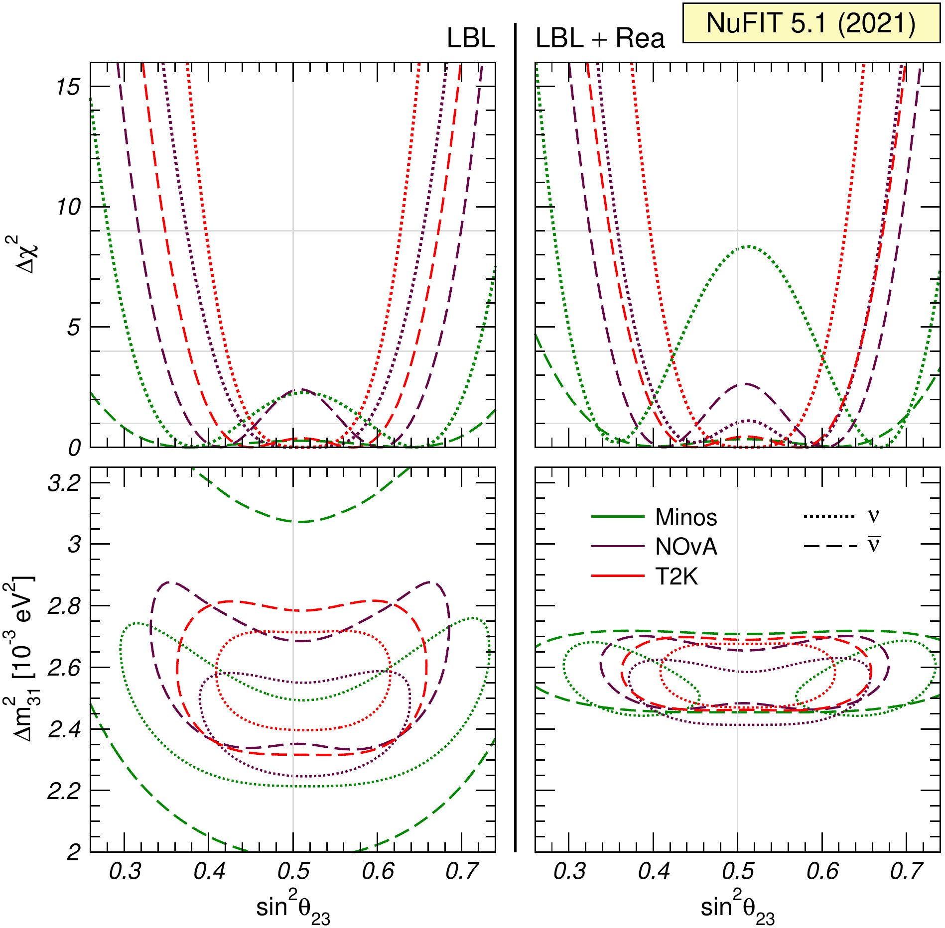
Bounds on θ23 (upper panels) and 2σ allowed regions in the (sin2θ23, Δm231) plane (lower panels) from the analysis of MINOS (green), NOνA (dark-redwood) and T2K (red) disappearance data assuming Normal Ordering. The dotted (dashed) lines correspond to neutrino (antineutrino) data. In the left panels a prior on θ13 has been imposed to account for reactor bounds, while in the right panels LBL and reactor data are consistently combined together. In all panels solar and KamLAND data are included to constrain Δm221 and θ12. |
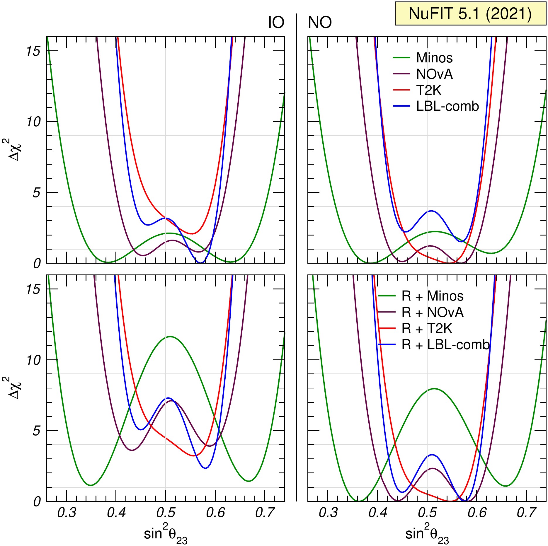
Synergies: determination of θ23
pdf jpg |
Bounds on θ23 from MINOS (green), NOνA (dark-redwood), T2K (red) and their combination (blue). Left (right) panels are for IO (NO); for each experiment Δχ2 is defined with respect to the global minimum of the two orderings. The upper panels show the 1-dimensional Δχ2 from LBL accelerator experiments after imposing a prior on θ13 to account for reactor bounds. The lower panels show the corresponding determination when the full information of LBL and reactor experiments is used in the combination. In all panels solar and KamLAND data are included to constrain Δm221 and θ12. |
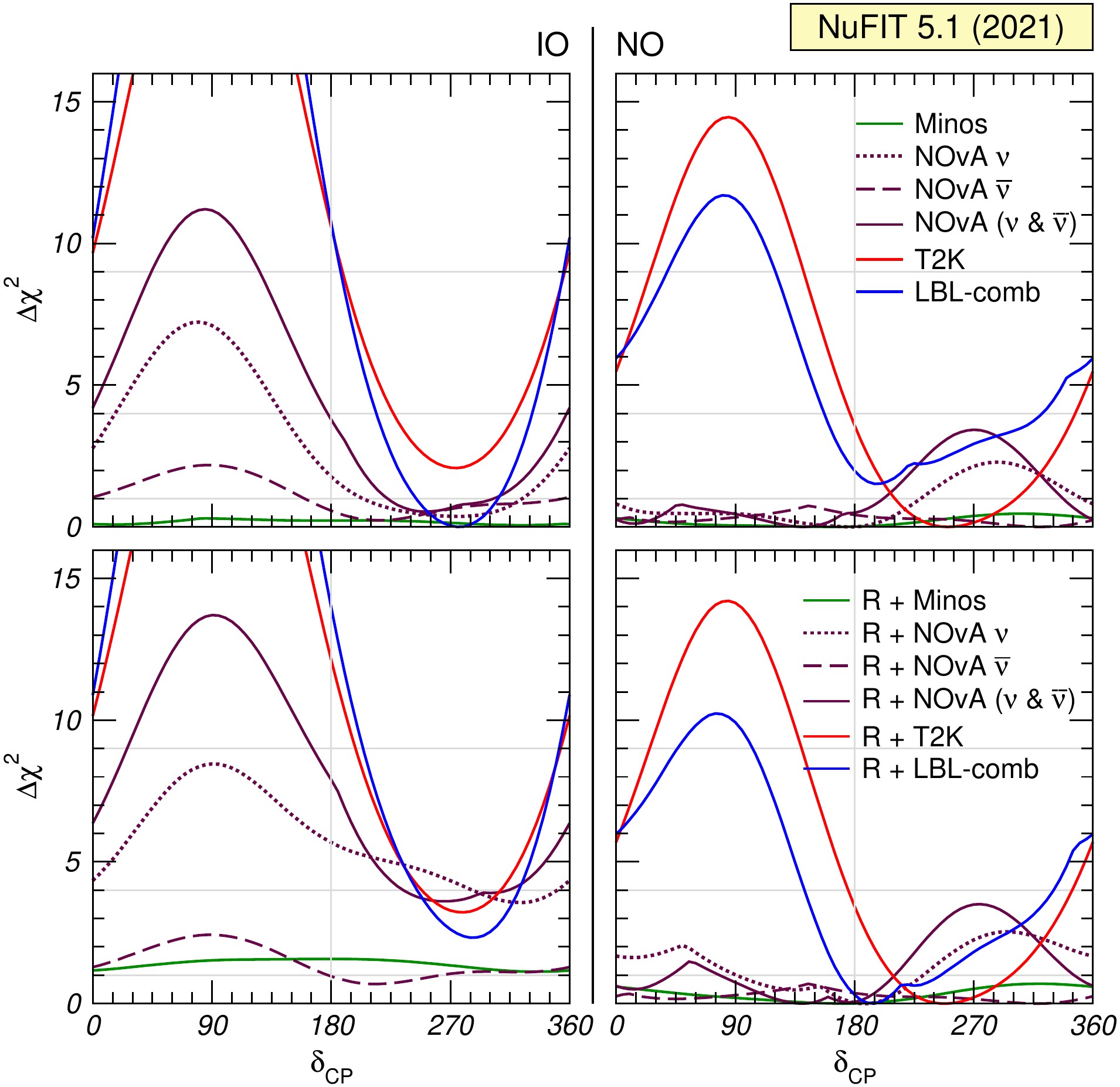
Synergies: determination of δCP
pdf jpg |
Bounds on δCP from MINOS (green), NOνA (dark-redwood), T2K (red) and their combination (blue). Left (right) panels are for IO (NO); for each experiment Δχ2 is defined with respect to the global minimum of the two orderings. For NOνA we also show as dotted (dashed) lines the results obtained using only neutrino (antineutrino) data. The upper panels show the 1-dimensional Δχ2 from LBL accelerator experiments after imposing a prior on θ13 to account for reactor bounds. The lower panels show the corresponding determination when the full information of LBL and reactor experiments is used in the combination. In all panels solar and KamLAND data are included to constrain Δm221 and θ12. |
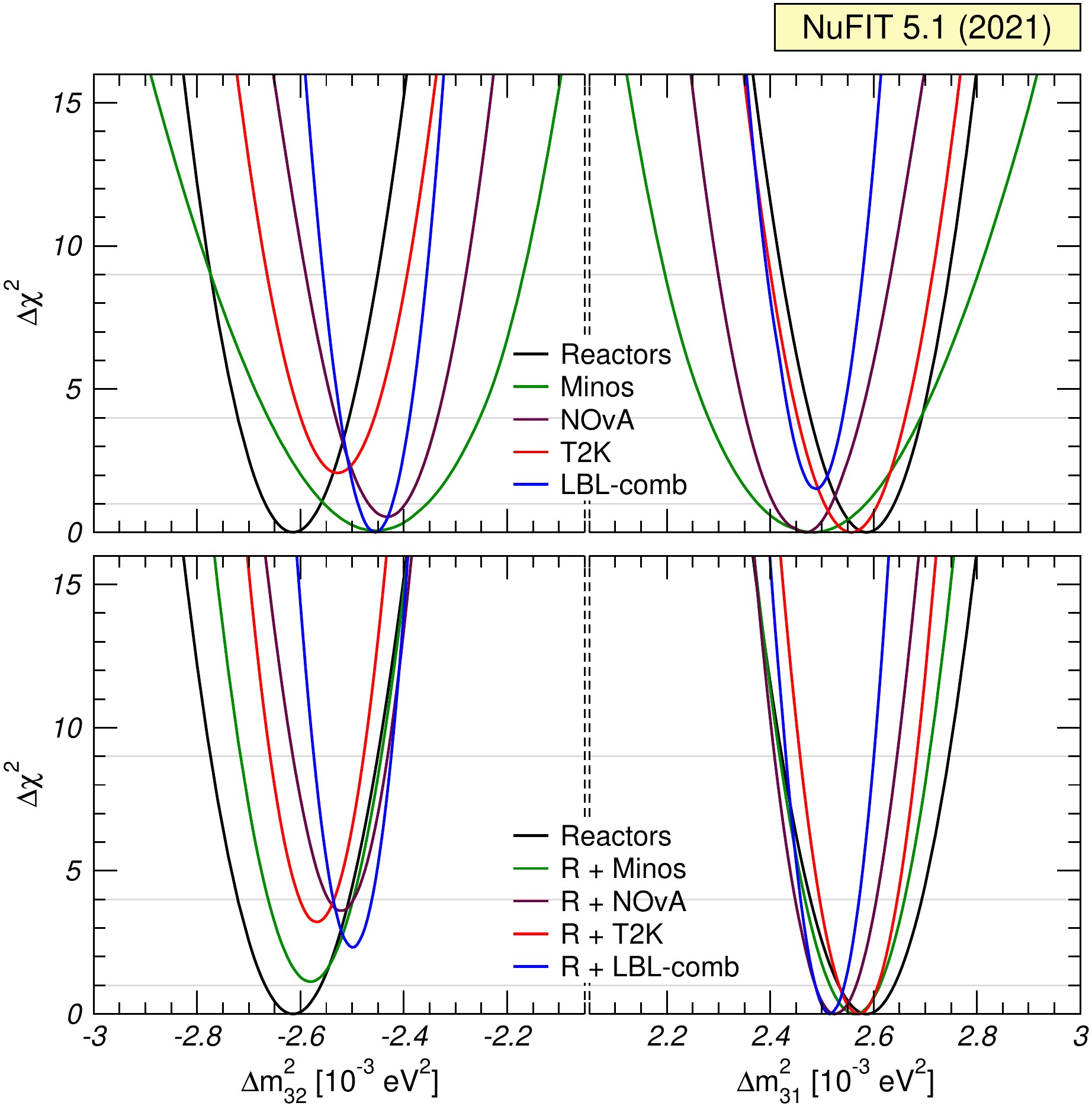
Synergies: determination of Δm23ℓ
pdf jpg |
Bounds on Δm23ℓ from reactor experiments (black) as well as MINOS (green), NOνA (dark-redwood), T2K (red) and all LBL data (blue). Left (right) panels are for IO (NO); for each experiment Δχ2 is defined with respect to the global minimum of the two orderings. The upper panels show the 1-dimensional Δχ2 from LBL accelerator experiments after imposing a prior on θ13 to account for reactor bounds. The lower panels show the corresponding determination when the full information of LBL and reactor experiments is used in the combination. In all panels solar and KamLAND data are included to constrain Δm221 and θ12. |
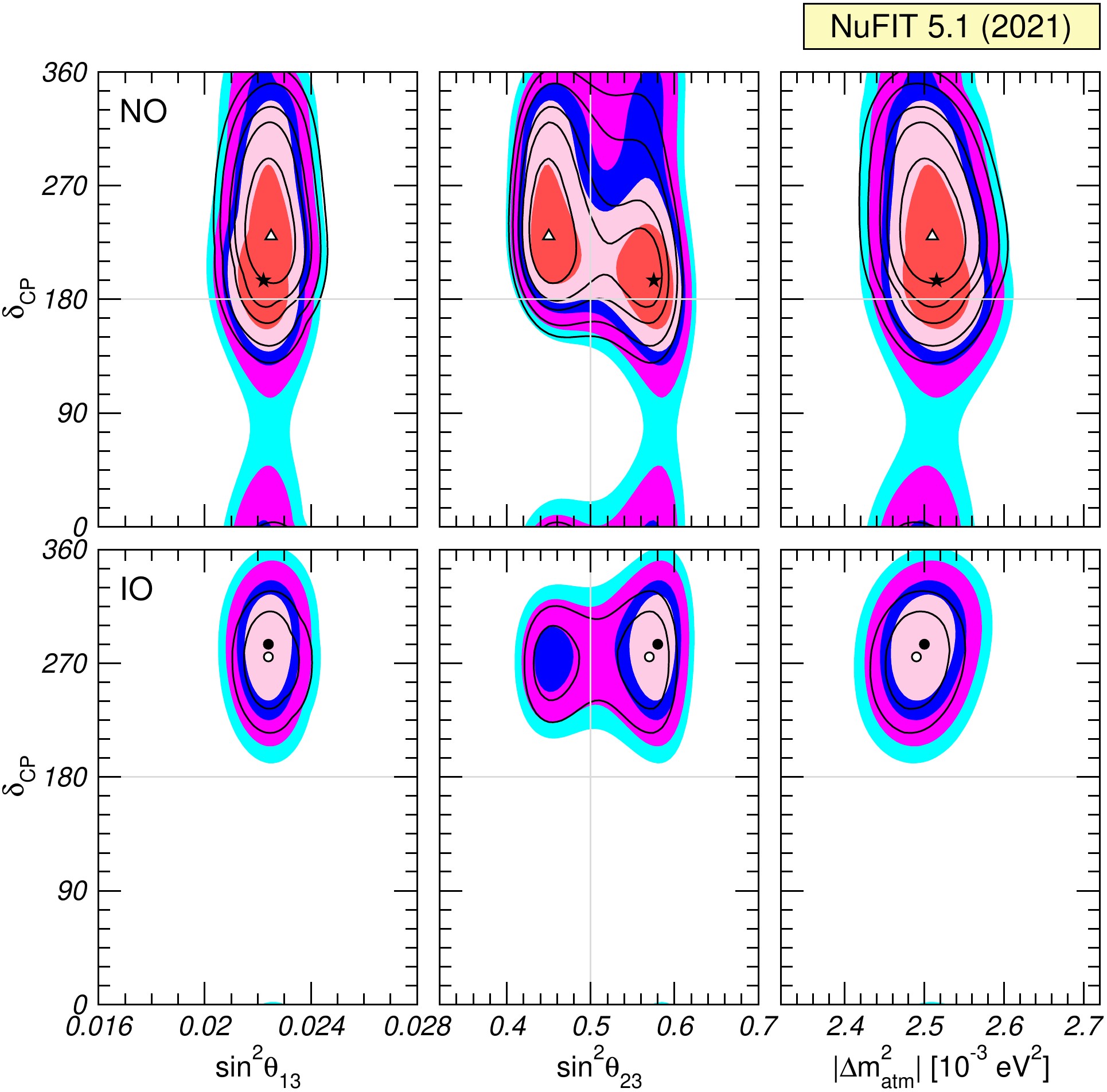
Correlation between δCP and other parameters
pdf jpg |
Allowed regions from the global analysis after minimizing with respect to all undisplayed parameters. The upper (lower) panel corresponds to IO (NO). Colored regions (black contour curves) are obtained without (with) the inclusion of the tabulated SK-atm χ2 data. The different contours correspond to the two-dimensional allowed regions at 1σ, 90%, 2σ, 99%, 3σ CL (2 dof). Note that as atmospheric mass-squared splitting we use Δm231 for NO and Δm232 for IO. |
| We provide one-, two- and three-dimensional Δχ2 projections for both the analysis without (Normal and Inverted Ordering) and including (Normal and Inverted Ordering) Super-Kamiokande atmospheric data. A description of the content of these files and a summary of the data included in our analysis can be found here. |
»