v1.1: Three-neutrino fit based on data available in March 2013
Menu
If you are using these results please refer to JHEP 12 (2012) 123 [arXiv:1209.3023] as well as NuFIT 1.1 (2013), www.nu-fit.org.
|
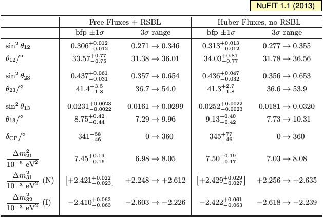
| Three-flavour oscillation parameters from our fit to global data as of March 2013. For "Free Fluxes + RSBL" reactor fluxes have been left free in the fit and short baseline reactor data (RSBL) with L shorter than ~100 m are included; for "Huber Fluxes, no RSBL" the flux prediction from arXiv:1106.0687 are adopted and RSBL data are not used in the fit. Numbers in brackets correspond to local minima. |
|
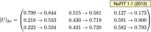
| 3σ CL ranges of the magnitude of the elements of the three-flavour leptonic mixing matrix under the assumption of the matrix U being unitary. The ranges in the different entries of the matrix are correlated due to the fact that, in general, the result of a given experiment restricts a combination of several entries of the matrix, as well as to the constraints imposed by unitarity. As a consequence choosing a specific value for one element further restricts the range of the others. |
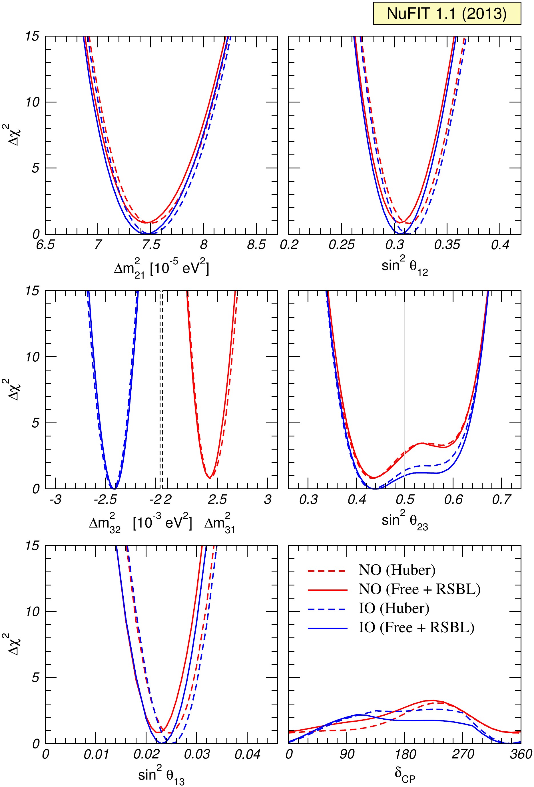
One-dimensional χ2 projections:
pdf jpg |
Global 3ν oscillation analysis. The red (blue) curves are for Normal (Inverted) Ordering. Results for different assumptions concerning the analysis of data from reactor experiments are shown: for solid curves the normalization of reactor fluxes is left free and data from short-baseline (less than 100 m) reactor experiments are included. For dashed curves short-baseline data are not included but reactor fluxes as predicted in arXiv:1106.0687 are assumed. Note that as atmospheric mass-squared splitting we use Δm231 for NO and Δm232 for IO. |
Two-dimensional allowed regions
pdf jpg |
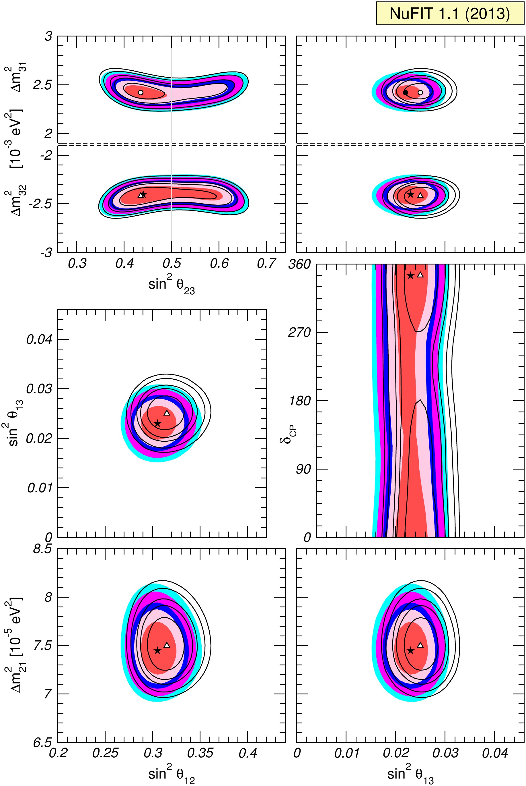
Global 3ν oscillation analysis. Each panel shows the two-dimensional projection of the allowed six-dimensional region after marginalization with respect to the undisplayed parameters. The different contours correspond to the two-dimensional allowed regions at 1σ, 90%, 2σ, 99%, 3σ CL (2 dof). Results for different assumptions concerning the analysis of data from reactor experiments are shown: full regions correspond to an analysis with the normalization of reactor fluxes left free and data from short-baseline (less than 100 m) reactor experiments are included. For void regions short-baseline reactor data are not included but reactor fluxes as predicted in arXiv:1106.0687 are assumed. Note that as atmospheric mass-squared splitting we use Δm231 for NO and Δm232 for IO. |
Contributions to the determination of θ13

pdf jpg |
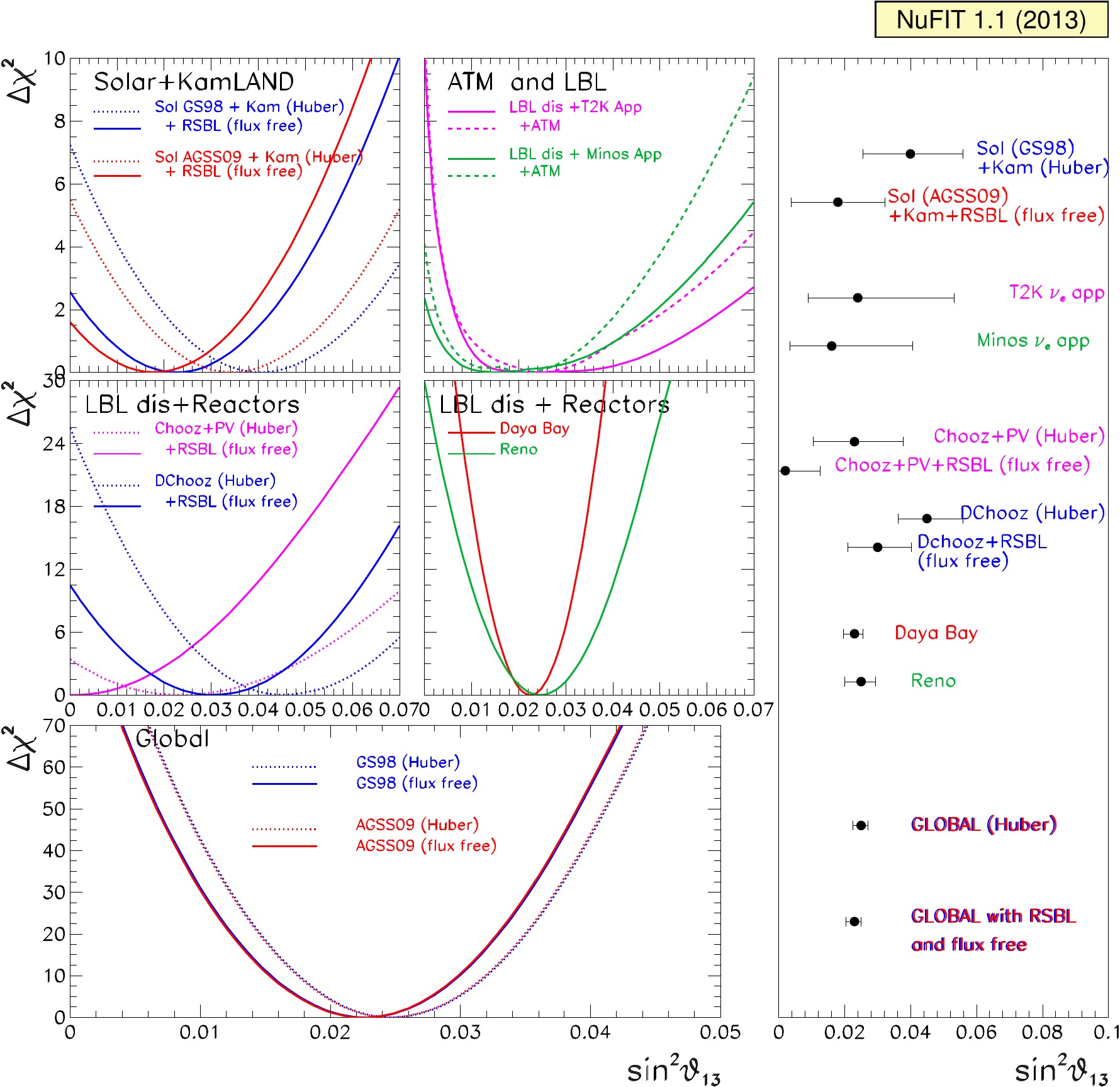
Dependence of Δχ2 on θ13 for the different data samples and assumptions quoted in each panel. In the right panel we show the corresponding 1σ ranges. |
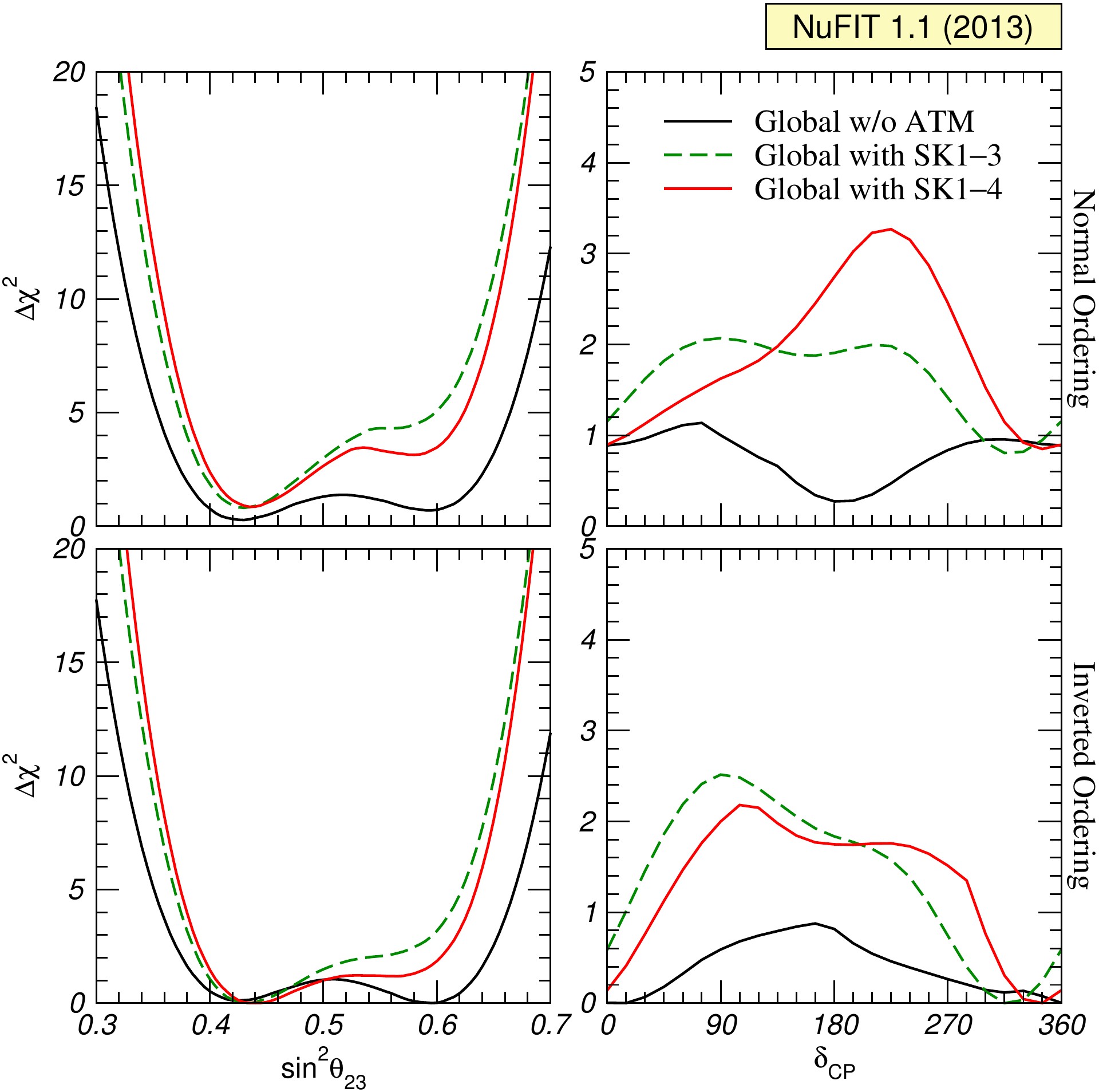
pdf jpg |
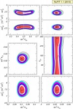
Δχ2 as a function of θ23 and δCP for three different analysis assumptions on the atmospheric data included as labeled in the figure. Upper (lower) panels correspond to Normal (Inverted) ordering. |
Correlation between δCP and other parameters
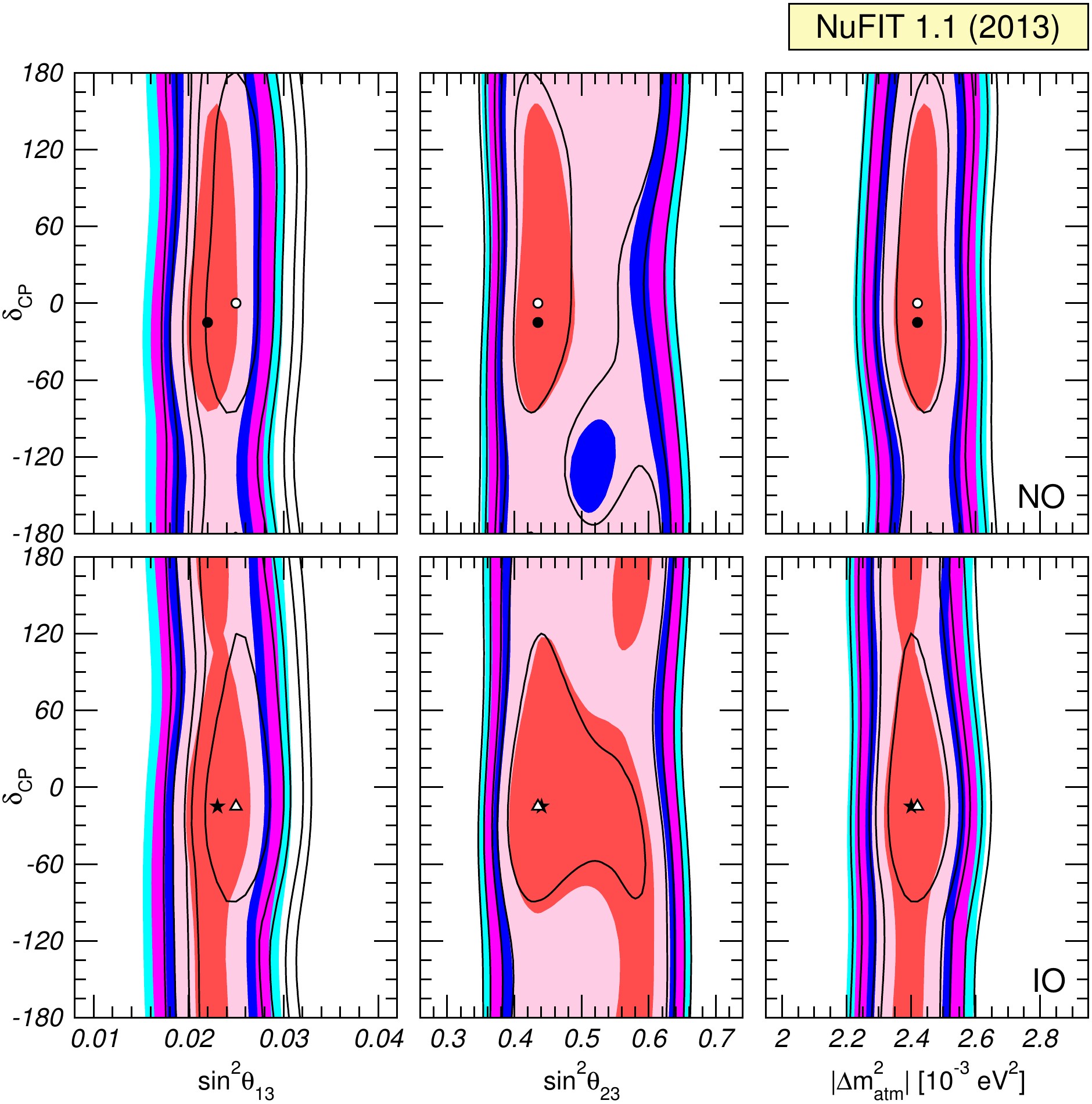
pdf jpg |
Global 3ν oscillation analysis. Each panel shows the two-dimensional projection of the allowed six-dimensional region after marginalization with respect to the undisplayed parameters. The different contours correspond to the two-dimensional allowed regions at 1σ, 90%, 2σ, 99%, 3σ CL (2 dof). Results for different assumptions concerning the analysis of data from reactor experiments are shown: full regions correspond to an analysis with the normalization of reactor fluxes left free and data from short-baseline (less than 100 m) reactor experiments are included. For void regions short-baseline reactor data are not included but reactor fluxes as predicted in arXiv:1106.0687 are assumed. Upper (lower) panels are for NO (IO). |
»