v1.3: Three-neutrino fit based on data available in June 2014
Menu
- Summary of data included
- Parameter ranges
- Leptonic mixing matrix
- One-dimensional χ2 projections
- Two-dimensional allowed regions
- Contributions to the determination of θ13
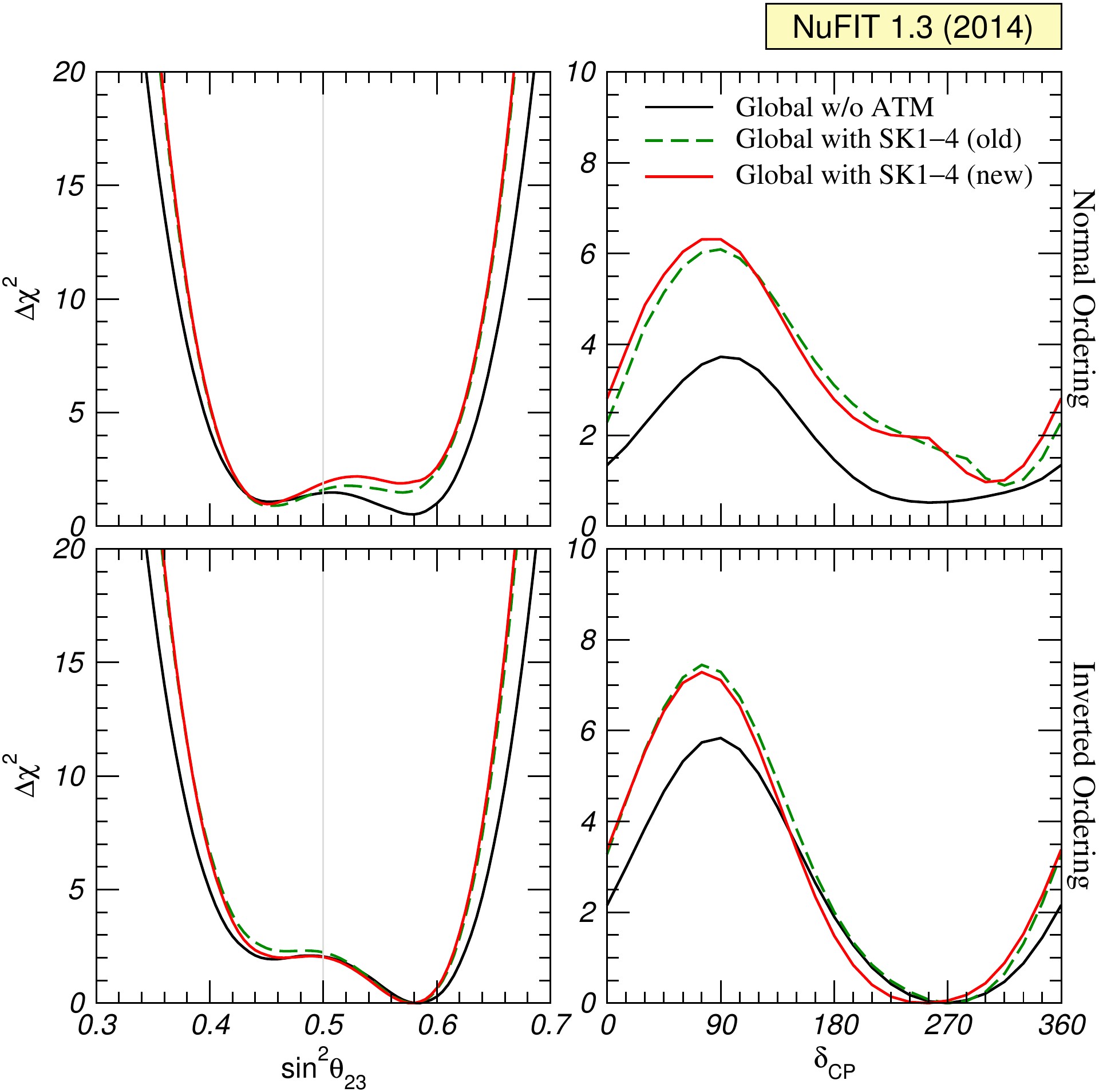
- Role of atmospheric neutrinos
- Correlation between δCP and other parameters
- CP violation: Jarlskog invariant and unitarity triangles
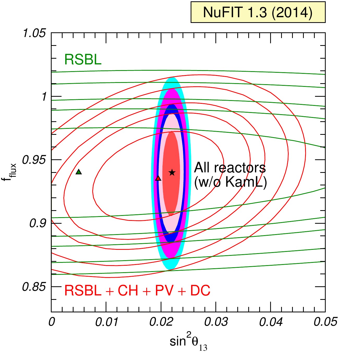
- Reactor fluxes
If you are using these results please refer to JHEP 12 (2012) 123 [arXiv:1209.3023] as well as NuFIT 1.3 (2014), www.nu-fit.org.
|
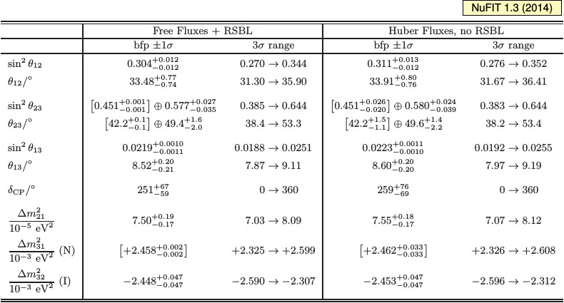
| Three-flavor oscillation parameters from our fit to global data as of June 2014. For "Free Fluxes + RSBL" reactor fluxes have been left free in the fit and short baseline reactor data (RSBL) with L shorter than ~100 m are included; for "Huber Fluxes, no RSBL" the flux prediction from arXiv:1106.0687 are adopted and RSBL data are not used in the fit. Note that 1σ and 3σ ranges are always given with respect to the global minimum. This leads to reduced intervals for local minima (enclosed in brackets), such as for Δm231 (NO) and for θ23 < 45°. |
|
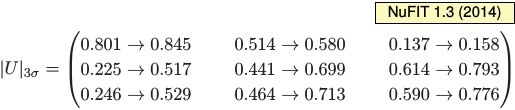
| 3σ CL ranges of the magnitude of the elements of the three-flavor leptonic mixing matrix under the assumption of the matrix U being unitary. The ranges in the different entries of the matrix are correlated due to the fact that, in general, the result of a given experiment restricts a combination of several entries of the matrix, as well as to the constraints imposed by unitarity. As a consequence choosing a specific value for one element further restricts the range of the others. |
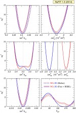
One-dimensional χ2 projections
pdf jpg |
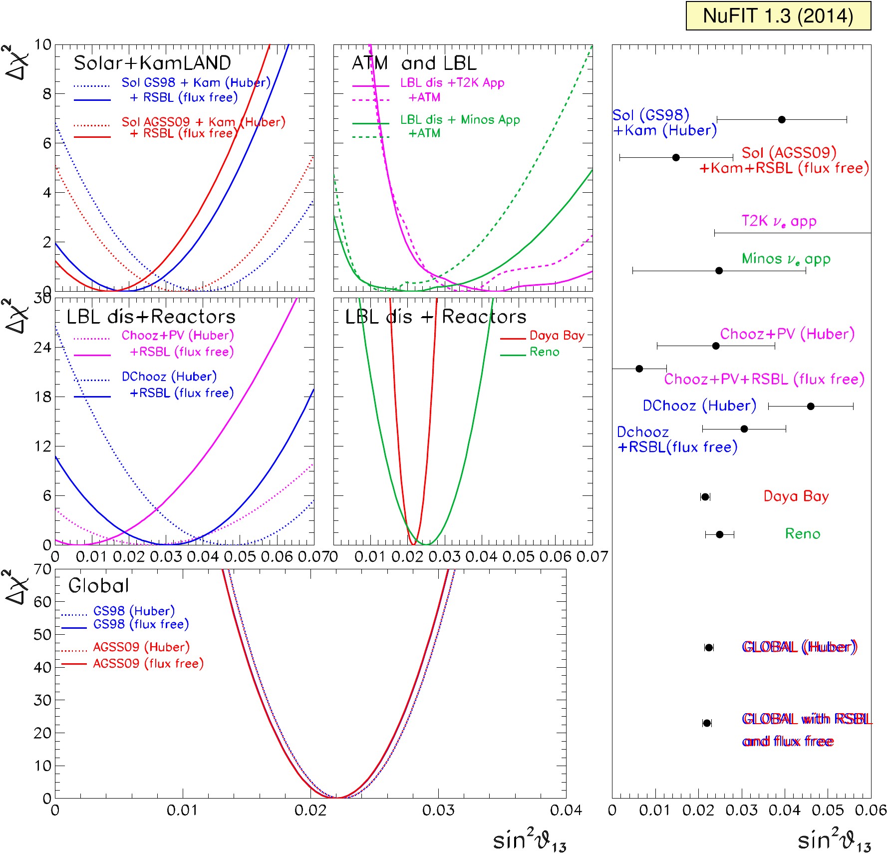
Global 3ν oscillation analysis. The red (blue) curves are for Normal (Inverted) Ordering. Results for different assumptions concerning the analysis of data from reactor experiments are shown: for solid curves the normalization of reactor fluxes is left free and data from short-baseline (less than 100 m) reactor experiments are included. For dashed curves short-baseline data are not included but reactor fluxes as predicted in arXiv:1106.0687 are assumed. Note that as atmospheric mass-squared splitting we use Δm231 for NO and Δm232 for IO. |
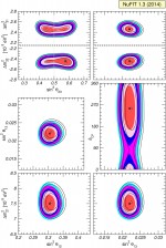
Two-dimensional allowed regions
pdf jpg |
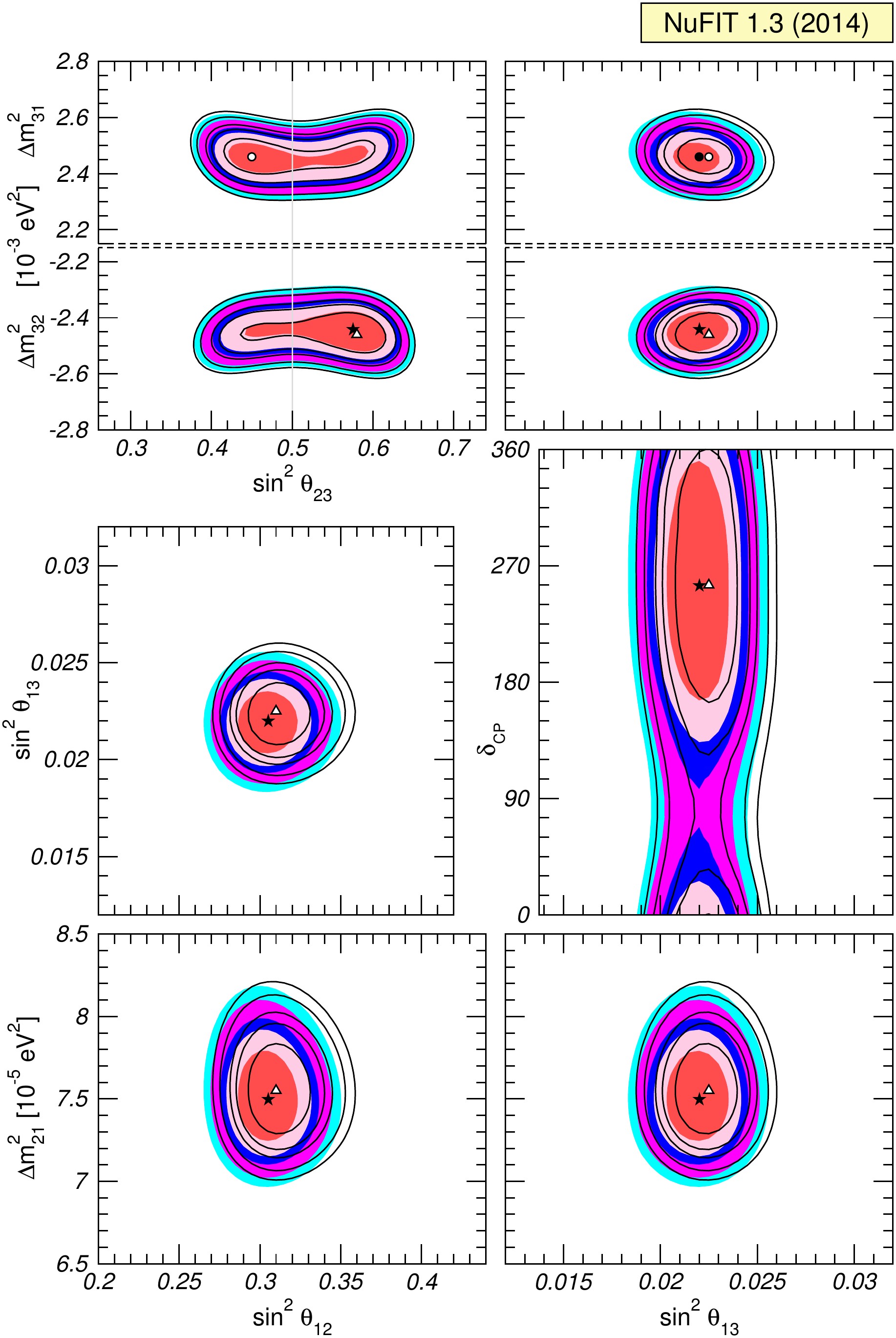
Global 3ν oscillation analysis. Each panel shows the two-dimensional projection of the allowed six-dimensional region after marginalization with respect to the undisplayed parameters. The different contours correspond to the two-dimensional allowed regions at 1σ, 90%, 2σ, 99%, 3σ CL (2 dof). Results for different assumptions concerning the analysis of data from reactor experiments are shown: full regions correspond to an analysis with the normalization of reactor fluxes left free and data from short-baseline (less than 100 m) reactor experiments are included. For void regions short-baseline reactor data are not included but reactor fluxes as predicted in arXiv:1106.0687 are assumed. Note that as atmospheric mass-squared splitting we use Δm231 for NO and Δm232 for IO. |
Contributions to the determination of θ13
pdf jpg |
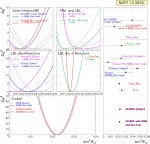
Dependence of Δχ2 on θ13 for the different data samples and assumptions quoted in each panel. In the right panel we show the corresponding 1σ ranges. |
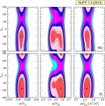
pdf jpg |
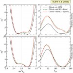
Δχ2 as a function θ23 and δCP for three different analysis assumptions on the atmospheric data included as labeled in the figure. Upper (lower) panels correspond to Normal (Inverted) ordering. |
Correlation between δCP and other parameters
pdf jpg |
Global 3ν oscillation analysis. Each panel shows the two-dimensional projection of the allowed six-dimensional region after marginalization with respect to the undisplayed parameters. The different contours correspond to the two-dimensional allowed regions at 1σ, 90%, 2σ, 99%, 3σ CL (2 dof). Results for different assumptions concerning the analysis of data from reactor experiments are shown: full regions correspond to an analysis with the normalization of reactor fluxes left free and data from short-baseline (less than 100 m) reactor experiments are included. For void regions short-baseline reactor data are not included but reactor fluxes as predicted in arXiv:1106.0687 are assumed. Upper (lower) panels are for NO (IO). |
CP-violation: Jarlskog invariant and unitarity triangles
pdf jpg |
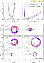
Upper panels: dependence of Δχ2 on the Jarlskog invariant. The red (blue) curves are for NO (IO). Results for different assumptions concerning the analysis of data from reactor experiments are shown: for solid curves the normalization of reactor fluxes is left free and data from short-baseline (less than 100 m) reactor experiments are included. For dashed curves short-baseline data are not included but reactor fluxes as predicted in arXiv:1106.0687 are assumed. Lower panels: the six leptonic unitarity triangles. After scaling and rotating each triangle so that two of its vertices always coincide with (0,0) and (1,0), we plot the 1σ, 90%, 2σ, 99%, 3σ CL (2 dof) allowed regions of the third vertex. Note that in the construction of the triangles the unitarity of the U matrix is always explicitly imposed. |
pdf jpg |
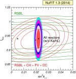
Allowed regions at 1σ, 90%, 2σ, 99%, 3σ CL (2 dof) in in the plane of θ13 and the flux normalization fflux (relative to the one predicted in arXiv:1106.0687) for the analysis of all reactor experiments CHOOZ, Palo Verde, Double-CHOOZ, Daya-Bay and RENO together with the reactor short-baseline experiments. In this figure we fix Δm231 to its best fit value. |
»