v2.0: Three-neutrino fit based on data available in September 2014
Menu
- Summary of data included
- Parameter ranges
- Leptonic mixing matrix
- Two-dimensional allowed regions
- One-dimensional χ2 projections
- CP-violation: Jarlskog invariant
- CP-violation: unitarity triangles
- Reactor fluxes
- Tension between Solar and KamLAND data
- Atmospheric mass-squared splitting
- Tendencies: contribution of different data
- Tendencies: correlation between δCP and θ23
- Tendencies: confidence levels on δCP
- Available data files
If you are using these results please refer to JHEP 11 (2014) 052 [arXiv:1409.5439] as well as NuFIT 2.0 (2014), www.nu-fit.org.
|
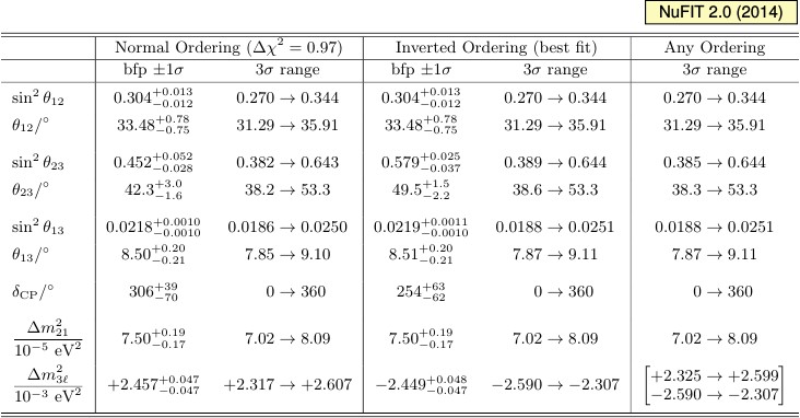
| Three-flavor oscillation parameters from our fit to global data as of September 2014. The results are presented for the "Free Fluxes + RSBL" in which reactor fluxes have been left free in the fit and short baseline reactor data (RSBL) with L shorter than ~100 m are included. The numbers in the 1st (2nd) column are obtained assuming NO (IO), i.e., relative to the respective local minimum, whereas in the 3rd column we minimize also with respect to the ordering. Note that Δm23ℓ = Δm231 > 0 for NO and Δm23ℓ = Δm232 < 0 for IO. |
|
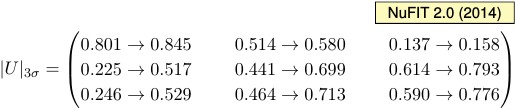
| 3σ CL ranges of the magnitude of the elements of the three-flavor leptonic mixing matrix under the assumption of the matrix U being unitary. The ranges in the different entries of the matrix are correlated due to the fact that, in general, the result of a given experiment restricts a combination of several entries of the matrix, as well as to the constraints imposed by unitarity. As a consequence choosing a specific value for one element further restricts the range of the others. |
Two-dimensional allowed regions
pdf jpg |
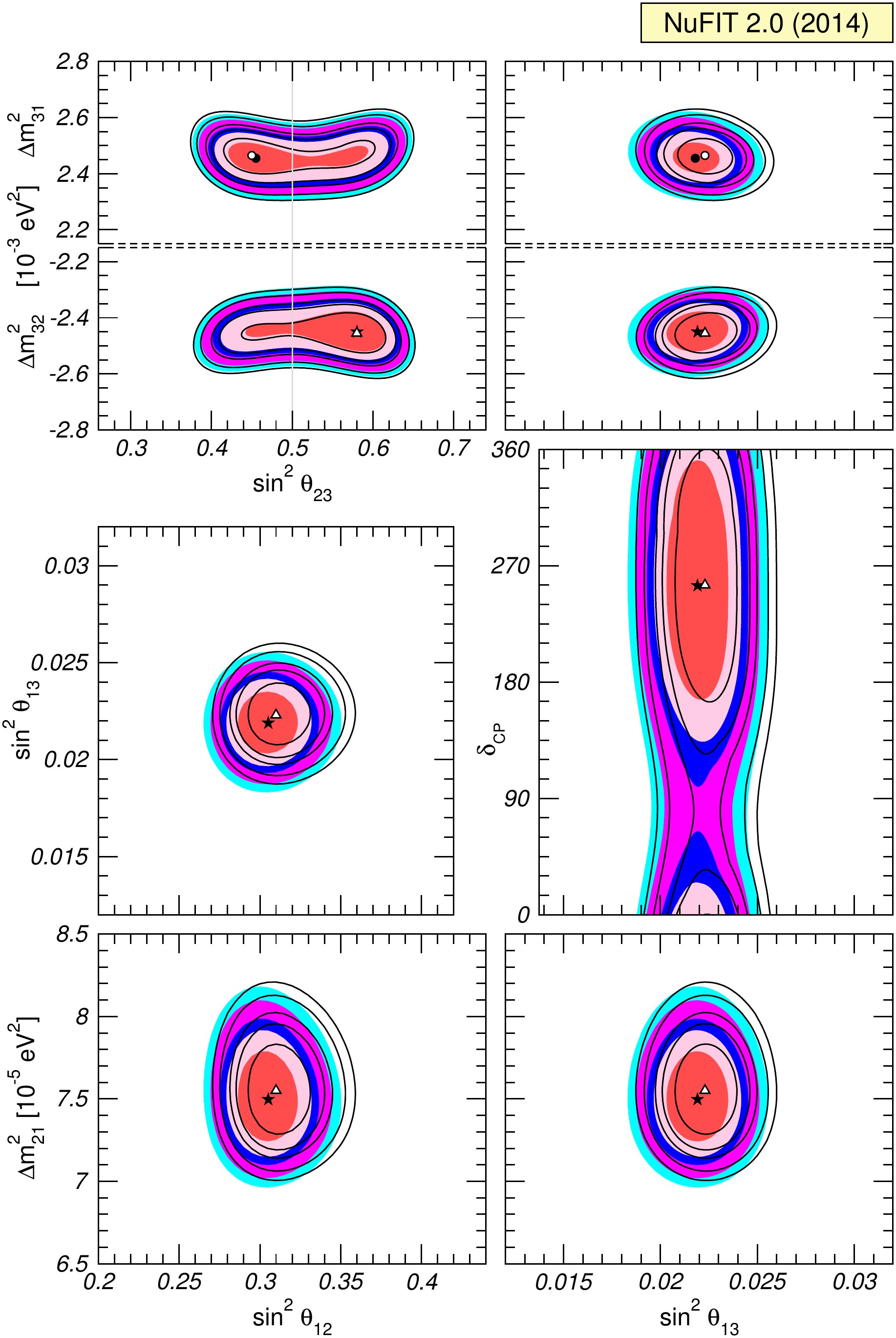
Global 3ν oscillation analysis. Each panel shows the two-dimensional projection of the allowed six-dimensional region after marginalization with respect to the undisplayed parameters. The different contours correspond to the two-dimensional allowed regions at 1σ, 90%, 2σ, 99%, 3σ CL (2 dof). Results for different assumptions concerning the analysis of data from reactor experiments are shown: full regions correspond to an analysis with the normalization of reactor fluxes left free and data from short-baseline (less than 100 m) reactor experiments are included. For void regions short-baseline reactor data are not included but reactor fluxes as predicted in arXiv:1106.0687 are assumed. Note that as atmospheric mass-squared splitting we use Δm231 for NO and Δm232 for IO. The regions in the lower 4 panels are based on a Δχ2 minimized with respect to the mass ordering. |
One-dimensional χ2 projections
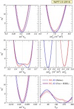
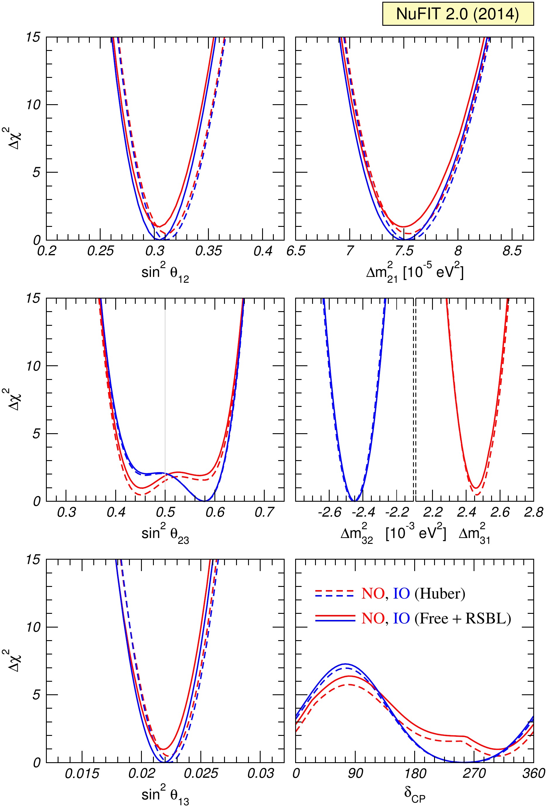
pdf jpg |
Global 3ν oscillation analysis. The red (blue) curves are for Normal (Inverted) Ordering. Results for different assumptions concerning the analysis of data from reactor experiments are shown: for solid curves the normalization of reactor fluxes is left free and data from short-baseline (less than 100 m) reactor experiments are included. For dashed curves short-baseline data are not included but reactor fluxes as predicted in arXiv:1106.0687 are assumed. Note that as atmospheric mass-squared splitting we use Δm231 for NO and Δm232 for IO. |
CP-violation: Jarlskog invariant
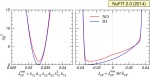
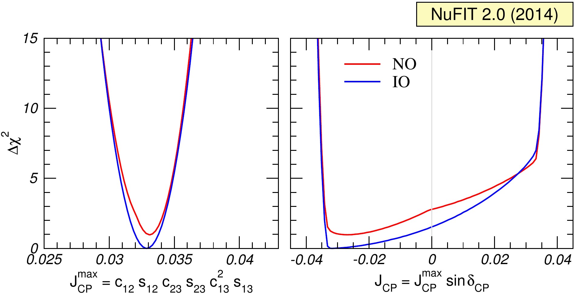
pdf jpg |
Dependence of Δχ2 on the Jarlskog invariant. The red (blue) curves are for NO (IO). The normalization of reactor fluxes is left free and data from short-baseline (less than 100 m) reactor experiments are included. |
CP-violation: unitarity triangles
pdf jpg |
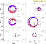
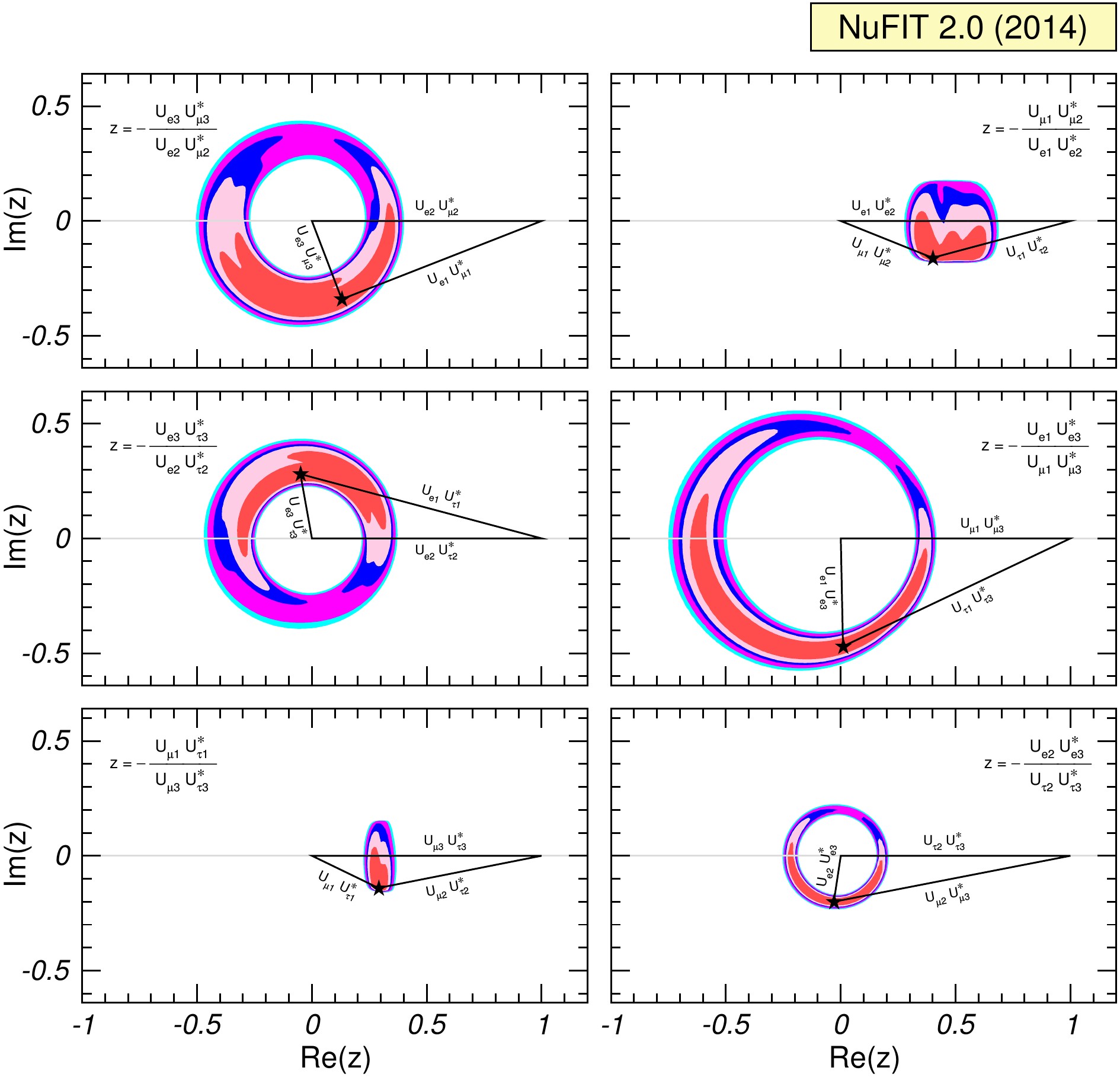
The six leptonic unitarity triangles. After scaling and rotating each triangle so that two of its vertices always coincide with (0,0) and (1,0), we plot the 1σ, 90%, 2σ, 99%, 3σ CL (2 dof) allowed regions of the third vertex. Note that in the construction of the triangles the unitarity of the U matrix is always explicitly imposed. |
pdf jpg |
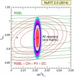
Allowed regions at 1σ, 90%, 2σ, 99%, 3σ CL (2 dof) in in the plane of θ13 and the flux reactor normalization fflux (relative to the one predicted in arXiv:1106.0687). Full regions correspond to the combined analysis of all reactor neutrino experiments with the exception of KamLAND, but including the RSBL experiments. The green contours correspond to only the RSBL experiments and red contours include RSBL + medium-baseline reactors without a near detector i.e., without including Daya-Bay and RENO. In this figure we fix Δm231 to its best fit value. |
Tension between Solar and KamLAND data

pdf jpg |
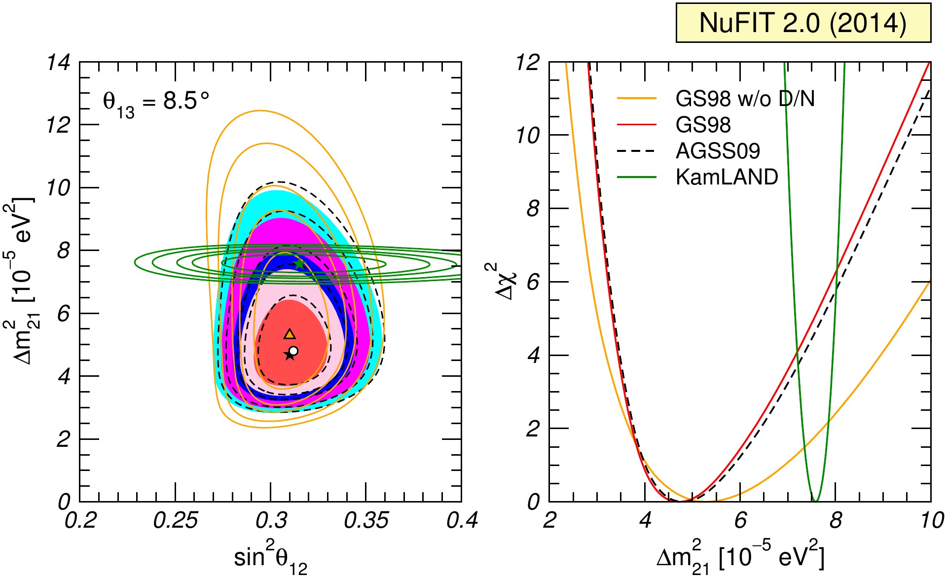
Left: Allowed parameter regions (at 1σ, 90%, 2σ, 99%, 3σ CL for 2 dof) from the combined analysis of solar data for GS98 model (full regions with best fit marked by black star) and AGSS09 model (dashed void contours with best fit marked by a white dot), and for the analysis of KamLAND data (solid green contours with best fit marked by a green star) for fixed θ13 = 8.5°. We also show as orange contours the results of a global analysis for the GS98 model but without including the day-night information from SK. Right: Δχ2 dependence on Δm221 for the same three analysis after marginalizing over θ12. |
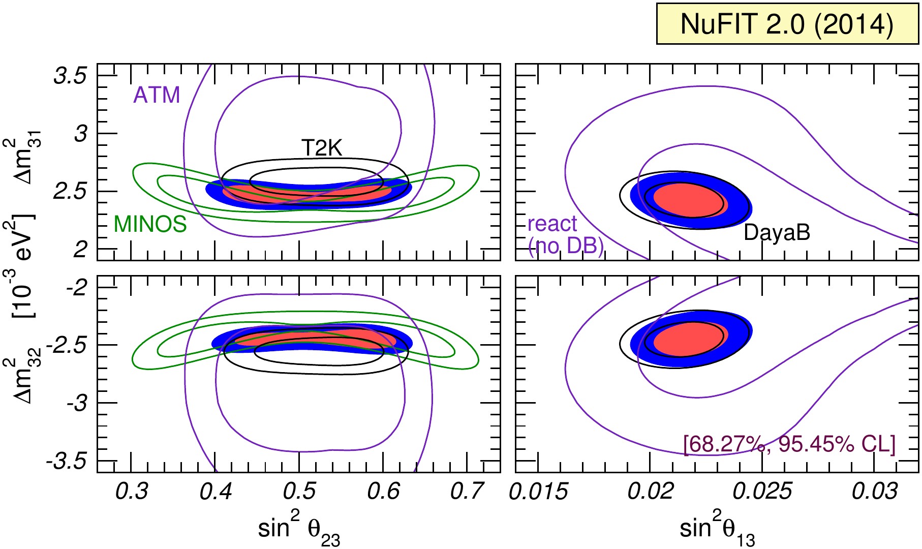
Atmospheric mass-squared splitting
pdf jpg |
Determination of Δm23ℓ at 1σ and 2σ (2 dof), where ℓ = 1 for NO (upper panels) and ℓ = 2 for IO (lower panels). The left panels show regions in the (sin2θ23, Δm23ℓ) plane using both appearance and disappearance data from MINOS (green) and T2K (black), as well as SK atmospheric data (violet) and a combination of them (colored regions). Here θ13 is constrained to the 3σ range from the global fit. The right panels show regions in the (sin2θ13, Δm23ℓ) plane using data from Daya-Bay (black), reactor data without Daya-Bay (violet), and their combination (colored regions). In all panels solar and KamLAND data are included to constrain Δm221 and θ12. Contours are defined with respect to the local minimum in each panel. |
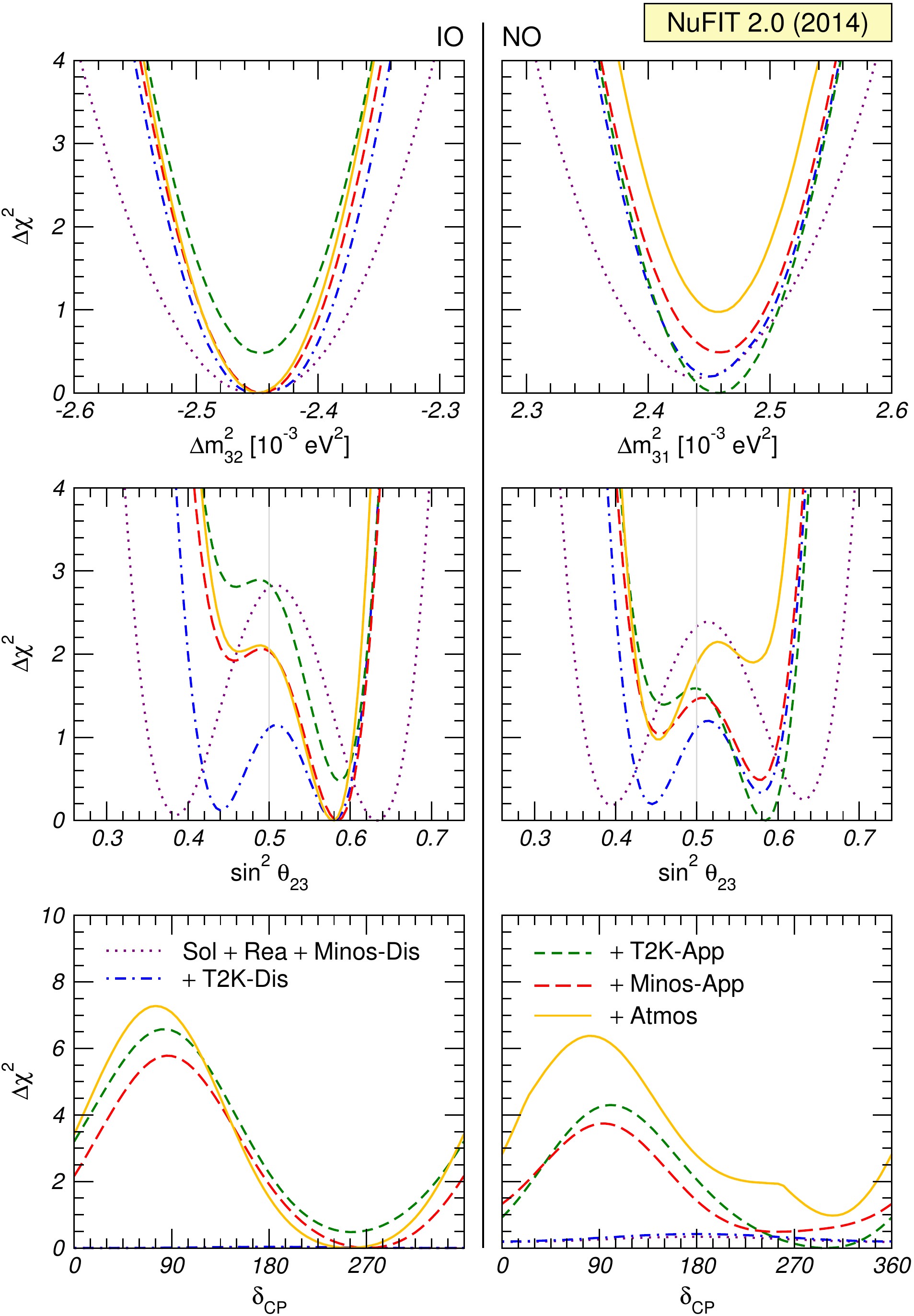
Tendencies: contribution of different data
pdf jpg |
Cumulative contribution of different sets of experimental results to the present tendencies in the determination of the mass ordering, the octant of θ23 and of the CP violating phase. Left (right) panels are for IO (NO). Violet (dotted): solar, reactor and MINOS νμ disappearance data. Blue (dot-dashed): same as violet, plus T2K νμ disappearance data. Green (short-dashed): same as blue, plus T2K νe appearance data. Red (long-dashed): same as green, plus MINOS νe appearance data. Orange (solid): same as red, plus Super-K atmospheric data (global fit). |
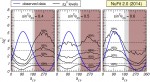
Tendencies: correlation between δCP and θ23
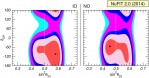
pdf jpg |
Allowed regions from the global data at 1σ, 90%, 2σ, 99%, 3σ CL (2 dof) in the (θ23, δCP) plane, after minimizing with respect to all undisplayed parameters. The left (right) panel corresponds to IO (NO). Contour regions in both panels are derived with respect to the global minimum which occurs for IO and is indicated by a star. The local minimum for NO is shown by a black dot. |
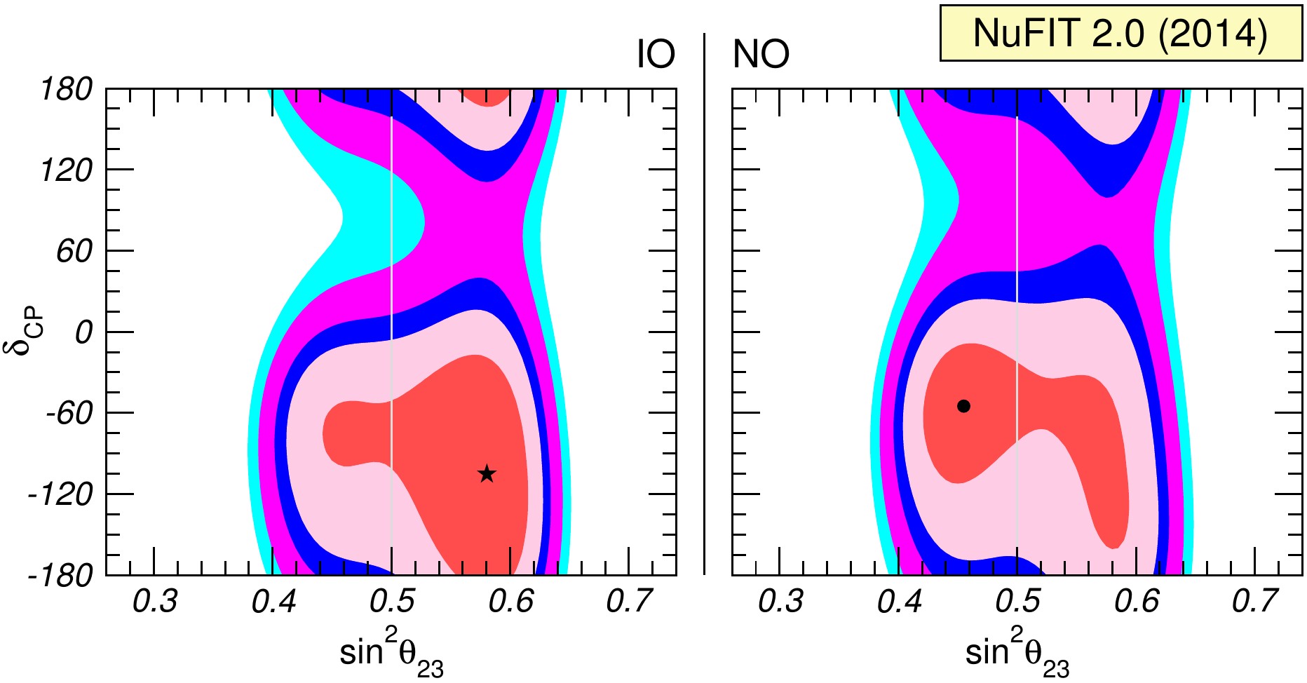
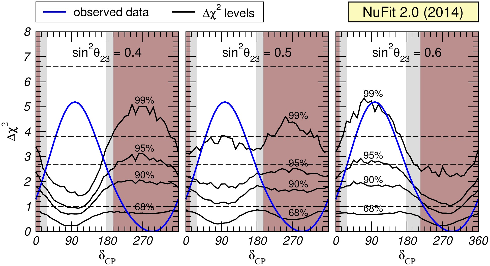
Tendencies: confidence levels on δCP
pdf jpg |
Black curves show the Δχ2 levels corresponding to 68%, 90%, 95%, 99% CL obtained from a Monte Carlo simulation of T2K appearance and disappearance data. Dashed lines correspond to the canonical values based on the χ2 distribution with 1 dof. The blue curve shows the observed Δχ2 using T2K data. The shaded regions indicate the 90% confidence interval for δCP based on the distribution from simulated pseudo-data (brown) and on the χ2 approximation (gray). The three panels correspond to different assumptions on the true value of θ23 used to generate the pseudo-data. In the fit all parameters except δCP and θ23 are fixed to the global best fit values, assuming normal mass ordering. |
»