v2.0: Bayesian analysis based on data available in September 2014
Menu
- Data summary (standard χ2 analysis)
- Parameter ranges
- Credible intervals: θ23
- Credible intervals: δCP
- Model comparison: θ23
- Model comparison: δCP
- Two-dimensional regions: Normal Ordering
- Two-dimensional regions: Inverted Ordering
- Two-dimensional regions: Mixed Ordering
- One-dimensional likelihoods: θ23
- One-dimensional likelihoods: δCP
- One-dimensional likelihoods: JCP
If you are using these results please refer to JHEP 09 (2015) 200 [arXiv:1507.04366] and JHEP 11 (2014) 052 [arXiv:1409.5439] as well as NuFIT 2.0 (2015), www.nu-fit.org.
|
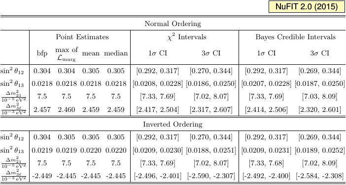
| Comparison of the results of χ2 and Bayesian analysis in the framework of three-flavor oscillations, using the global data available up to September 2014. Note that Δm23ℓ = Δm231 > 0 for NO and Δm23ℓ = Δm232 < 0 for IO. |
|
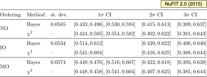
| Standard deviations, credible intervals, and χ2 intervals for sin2θ23. NO, IO and MO denote Normal Ordering, Inverted Ordering, and no assumption on the mass ordering, respectively. |
|
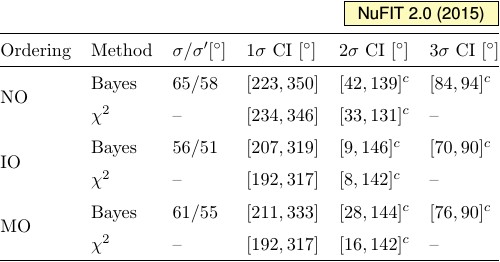
| Measures of dispersion, credible intervals, and χ2 intervals for δCP. Here [...]c is the complement of the interval [...], i.e., all values of δCP not contained in [...]. NO, IO and MO denote Normal Ordering, Inverted Ordering, and no assumption on the mass ordering, respectively. |
|
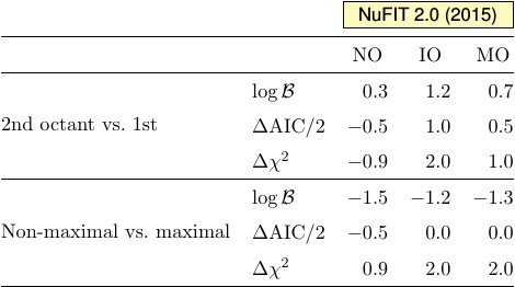
| Model comparison for different assumptions on sin2θ23. We list the logarithms of Bayes factors, the comparable differences in the Akaike Information Criterion (AIC), and the differences in χ2 minima. The sign is chosen such that positive values correspond to preference for first mentioned assumptions in each case, i.e., the 2nd octant and non-maximal mixing, respectively. |
|
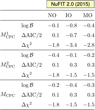
| Model comparson for different assumptions on δCP: M1CPC ≡ {δCP=0°}, M2CPC ≡ {δCP=180°}, MCPC ≡ {M1CPC ∨ M2CPC} with equal priors, and MCPV ≡ {δCP ∈ [0°, 360°] ∖ MCPC} with prior π(δCP) = 1/360°. We list the logarithms of Bayes factors relative to MCPV, the comparable differences in the Akaike Information Criterion (AIC), and the differences in χ2 as Δχ2 = χ2(MCPV) - χ2(MiCPC). For all variables, positive values would indicate preference of the corresponding MiCPC over MCPV. |
Two-dimensional regions: Normal Ordering

pdf jpg |
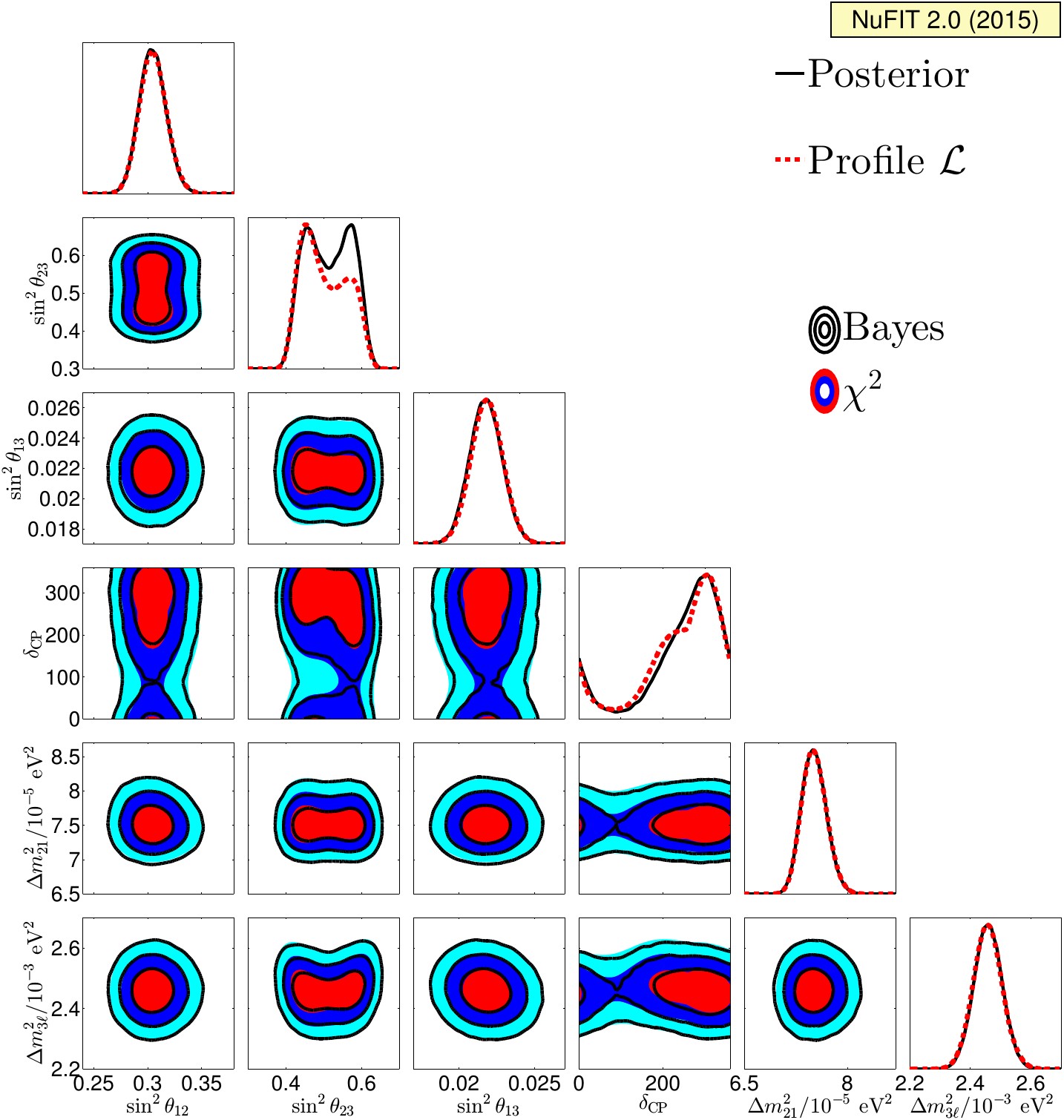
One-dimensional posterior distributions (black full lines) and two-dimensional 1σ, 2σ and 3σ Bayesian credible regions (black void contours) assuming Normal Ordering. The figure also shows the one-dimensional profile likelihoods (red dashed curves) and two-dimensional χ2 regions (colored filled regions) from the standard χ2 analysis. |
Two-dimensional regions: Inverted Ordering

pdf jpg |
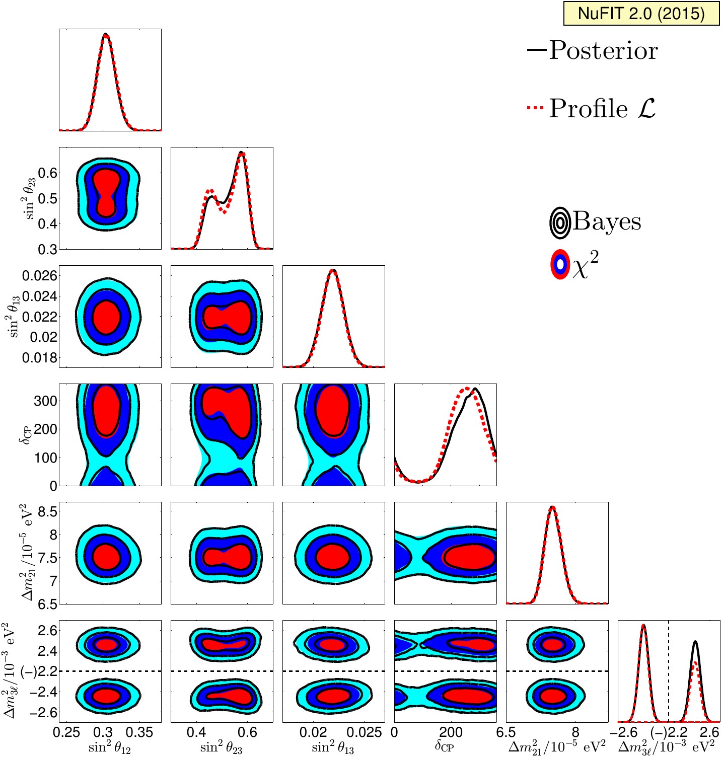
One-dimensional posterior distributions (black full lines) and two-dimensional 1σ, 2σ and 3σ Bayesian credible regions (black void contours) assuming Inverted Ordering. The figure also shows the one-dimensional profile likelihoods (red dashed curves) and two-dimensional χ2 regions (colored filled regions) from the standard χ2 analysis. |
Two-dimensional regions: Mixed Ordering

pdf jpg |
One-dimensional posterior distributions (black full lines) and two-dimensional 1σ, 2σ and 3σ Bayesian credible regions (black void contours) without any assumption on the mass ordering. The figure also shows the one-dimensional profile likelihoods (red dashed curves) and two-dimensional χ2 regions (colored filled regions) from the standard χ2 analysis. |
One-dimensional likelihoods: θ23
pdf jpg |
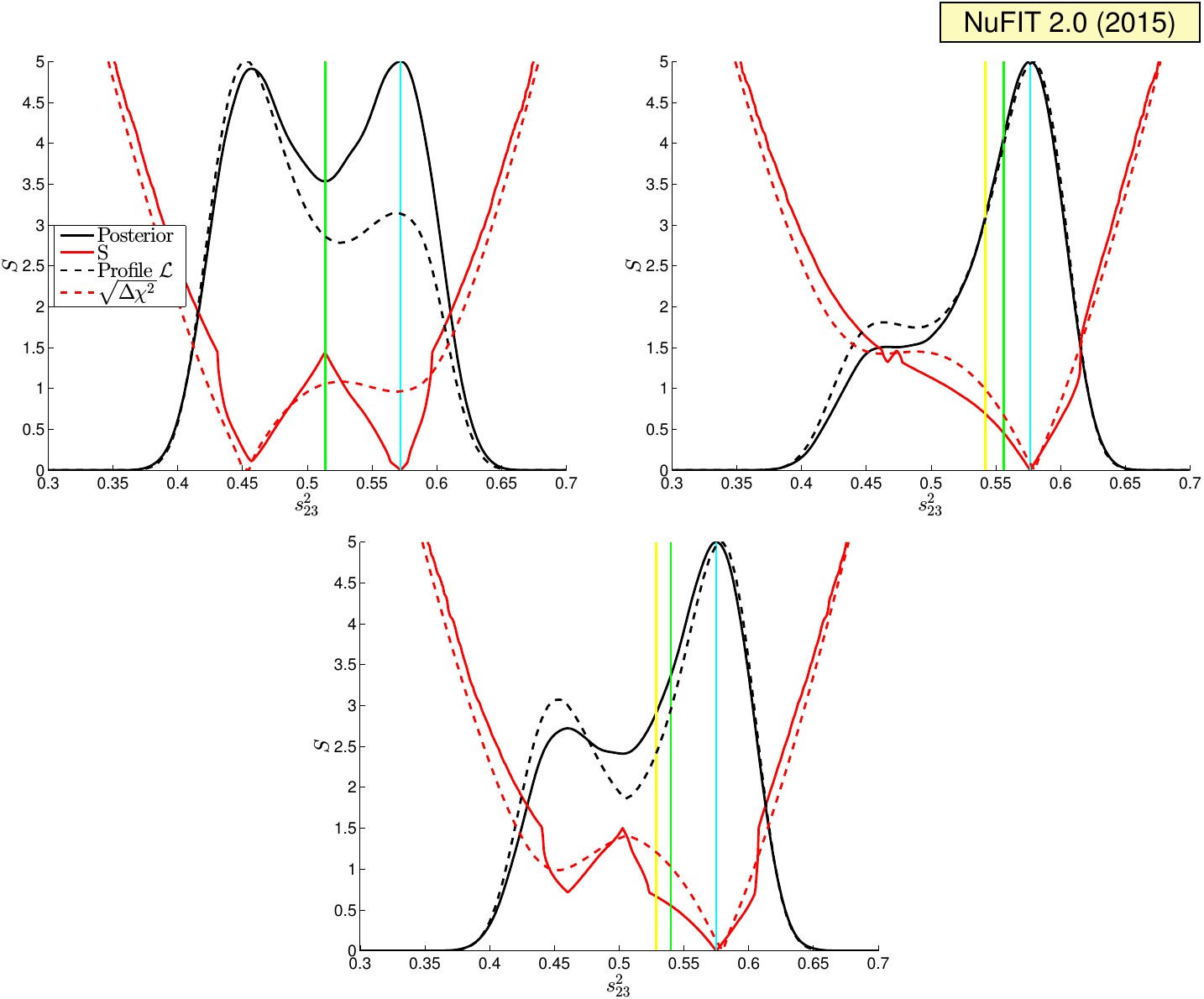
Bayesian posterior/marginal likelihood (black solid) and profile likelihood (black dashed) from the standard χ2 analysis, both normalized to their maximal value. We also plot the number of σ's (red solid) and √Δχ2 (red dashed) functions. The vertical lines show the posterior mean (yellow), the median (green), and the maximum of the marginal likelihood (cyan). The different panels correspond to Normal Ordering (top left), Inverted Ordering (top right) and Mixed Ordering (bottom). |
One-dimensional likelihoods: δCP
pdf jpg |
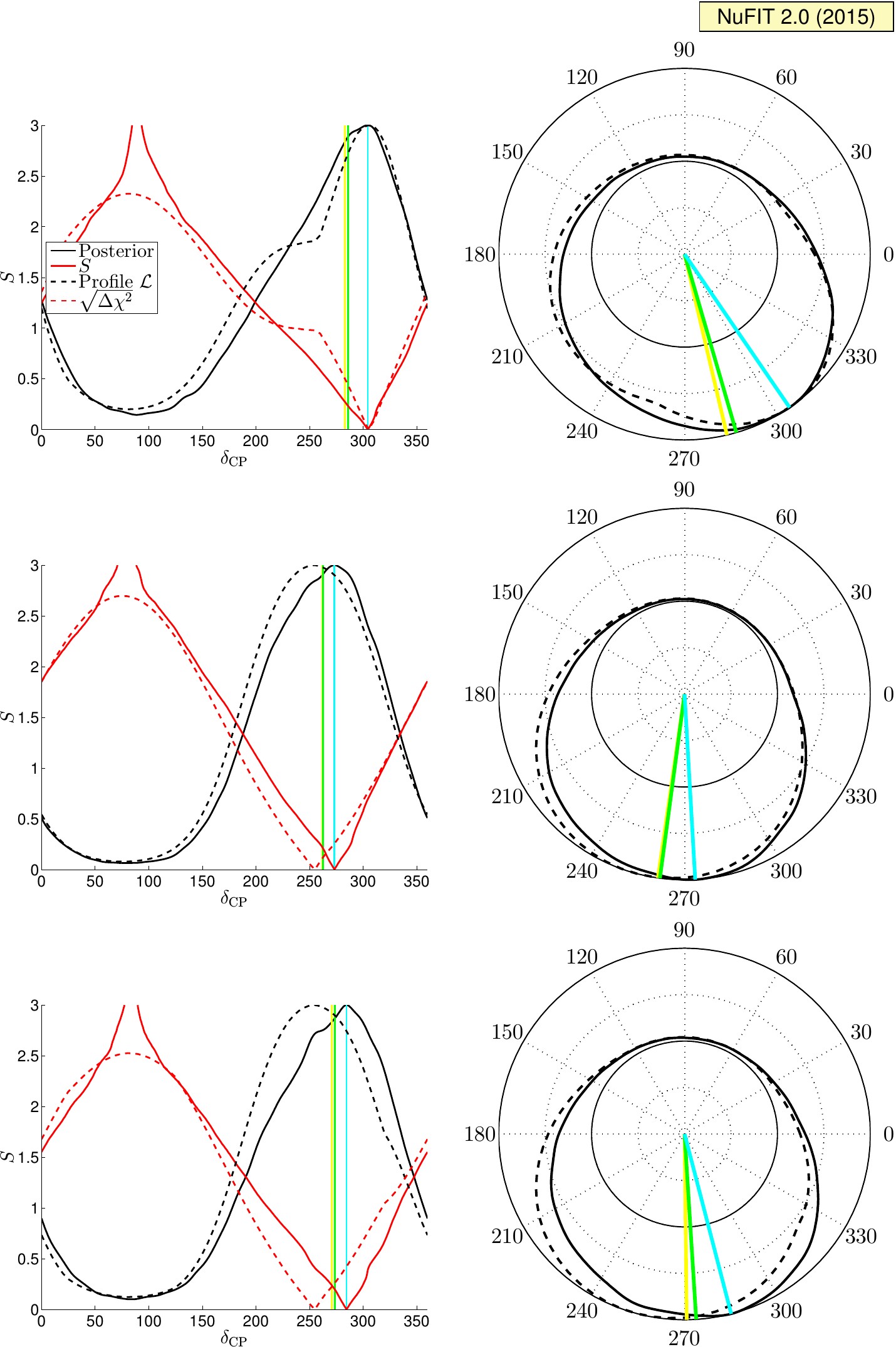
Bayesian posterior/marginal likelihood (black solid), profile likelihood (black dashed), number of σ's (red solid) and √Δχ2 (red dashed) as a function of δCP. The vertical lines show the posterior mean (yellow), the median (green), and the maximum of the marginal likelihood (cyan). The different panels correspond to Normal Ordering (top), Inverted Ordering (middle) and Mixed Ordering (bottom), both in cartesian (left) and polar (right) coordinates. |
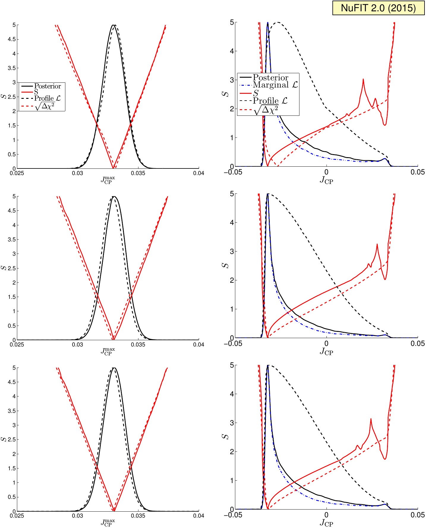
One-dimensional likelihoods: JCP
pdf jpg |
Bayesian posterior likelihood (black solid), profile likelihood (black dashed) and marginal likelihood (blue dot-dashed), together with the number of σ's (red solid) and √Δχ2 (red dashed) as a function of JCP (right) and its maximum value (left). The different panels correspond to Normal Ordering (top), Inverted Ordering (middle) and Mixed Ordering (bottom). |
»